- Home
- Assessments
- Bioregional Assessment Program
- Gloucester subregion
- 2.6.2 Groundwater numerical modelling for the Gloucester subregion
- 2.6.2.8 Uncertainty analysis
- 2.6.2.8.1 Quantitative uncertainty analysis
The workflow of the uncertainty analysis (see Section 2.6.2.1 and submethodology M09 (as listed in Table 1) for propagating uncertainty through models (Peeters et al., 2016)) starts with defining the prior parameter distributions. These are subsequently constrained by the available observations through Markov chain Monte Carlo sampling to generate the posterior parameter ensembles. These posterior parameter ensembles are then sampled to generate the ensembles of predictions.
2.6.2.8.1.1 Prior parameter distributions
Analytic element model
Table 8 Prior parameter distributions for the regional analytic element groundwater model
Data: Bioregional Assessment Programme (Dataset 1)
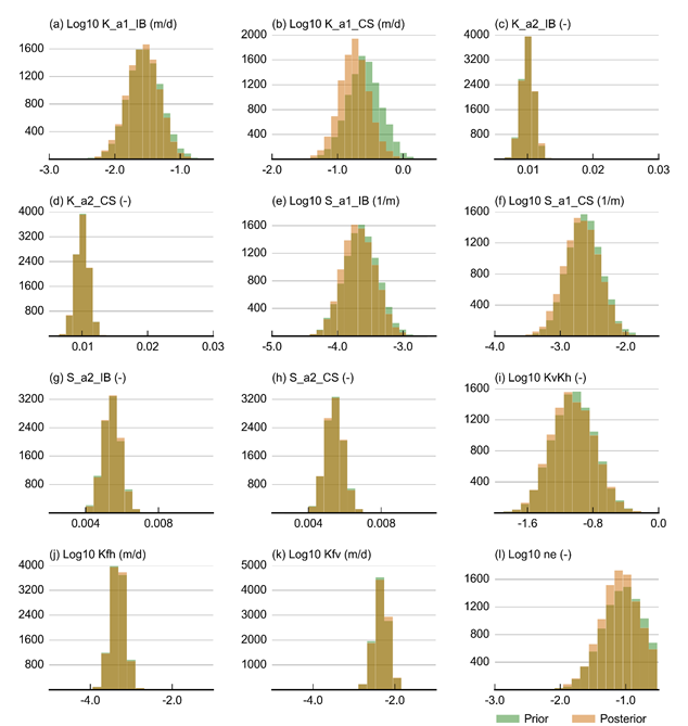
The factors included in the formal uncertainty analysis for the regional analytic element groundwater model (GW AEM) are the parameters listed in Table 5 in Section 2.6.2.6. The specification of the prior parameter distributions, shown in Table 8, was mostly driven by the geology and hydrogeology information presented in the context statement (companion product 1.1 for the Gloucester subregion (McVicar et al., 2014)). Figure 34 shows the prior distributions of each individual parameter.
All parameters are chosen to be normally distributed, either on the log scale or on the natural scale. The distribution for the intercepts of K (hydraulic conductivity) and S (storage) for interburden and coal seams (K_IB_intercept, K_CS_intercept, S_IB_intercept, S_CS_intercept) is chosen to be centred around the middle of the design of experiment range (Table 5) with a variance that ensures at least 99% of the probability mass of the prior distribution is within the bounds of the parameter range.
The slopes of the depth–hydraulic property relationship are chosen at the lower end of the range in Table 5, for both interburden and coal seams and for K and S. This ensures that when the depth–hydraulic property is evaluated, for the majority of the prior distributions, K and S values throughout the model domain are above the lower threshold values for hydraulic conductivity and storage (1 x 10⁻⁶ m/day and 1 x 10⁻⁷, respectively) defined in Section 2.6.2.6. As the relationship between the log of coal seam hydraulic conductivity and simulated coal seam gas (CSG) water production is linear (Figure 24 in Section 2.6.2.7.3), this choice of prior distributions will exclude very low CSG water production rates. This will lead to an overestimation rather than underestimation of hydrological change.
The ratio between horizontal and vertical K is chosen to be normally distributed on a log10 scale, centred in the middle of the Latin Hypercube sampling (LHS) range with a variance that ensures the prior distribution of the KvKh ratio spans an order of magnitude and that at least 99% of the probability mass of the prior distribution is within the bounds of the parameter range. The variances of the fault hydraulic conductivities are also chosen to span an order of magnitude, where the mean for the horizontal hydraulic conductivity is at the lower end of the LHS spectrum and the mean for the vertical hydraulic conductivity is at the higher end. While there are very few observations to justify these prior distributions, this choice of prior distribution is inspired by the precautionary principle as low horizontal fault hydraulic conductivity and high vertical fault hydraulic conductivity increases the potential propagation of the CSG depressurisation to the surface weathered and fractured rock layer.
The effective porosity of the leaky layer on top of the model is chosen to be centred on 0.1 with a variance that ensures at least 99% of the probability mass of the prior distribution is within the bounds of the parameter range.
Table 9 Variance – covariance matrix of the prior distributions of the analytic element model
Source: Bioregional Assessment Programme (Dataset 1)
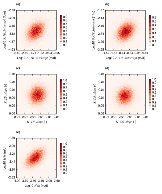
For five parameter combinations a covariance is specified as well (Table 9 and Figure 35). A covariance is defined between K_IB_intercept and S_IB_intercept, K_CS_intercept and S_CS_intercept, K_IB_slope and S_IB_slope, and K_CS_slope and S_CS_slope. There are insufficient joint measurements of hydraulic conductivity and storage to empirically establish these covariance rates. The covariance specified is based on a trial-and-error process design to decrease the likelihood of sampling unrealistic parameter combinations (high K – low S or vice versa) that lead to non-converging model runs (Figure 23, Section 2.6.2.7.3).
Covariance is also defined for the vertical and horizontal fault hydraulic conductivity. While these properties are not correlated, the covariance is specified to ensure that vertical fault hydraulic conductivity is more likely to be higher than the horizontal fault hydraulic conductivity. While this is not inspired by the observed fault-related flow in the basin, it adheres to the conceptualisation of faults as barriers of flow horizontally and conduits vertically.
The extent of the x-axis in each plot corresponds to the range of parameters sampled during the design of experiment. Refer to Table 5 in Section 2.6.2.6.1 for definitions of terms.
Data: Bioregional Assessment Programme (Dataset 1)
The colour scale is proportional to the density of points. Refer to Table 5 in Section 2.6.2.6.1 for definitions of terms.
Data: Bioregional Assessment Programme (Dataset 1)
Alluvial MODFLOW models
Table 10 Prior parameter distributions specified for the Avon and Karuah MODFLOW models
ascale parameter for Weibull distribution
bshape parameter for Weibull distribution
See Table 6 in Section 2.6.2.6.2 for definition and description of parameters.
Data: Bioregional Assessment Programme (Dataset 2)
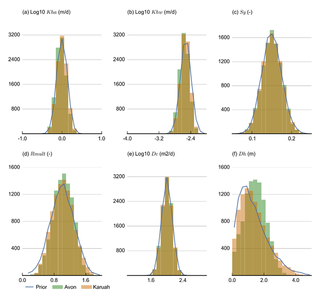
The factors included in the formal uncertainty analysis are the parameters listed in Table 10. The specification of the prior parameter distributions was mostly driven by the geology and hydrogeology information presented in the contextual statement (companion product 1.1 for the Gloucester subregion (McVicar et al., 2014)) and the data analysis (companion product 2.1-2.2 (Frery et al., 2018)). Figure 36 shows the prior distributions of each individual parameter.
The means of the prior parameter distributions are chosen to coincide with the centre of the range sampled in the design of experiment. The standard deviations are chosen to ensure at least 99% of the probability mass is within the range used in the design of experiment. The exception is Khw, for which the mean is chosen at the high end of the range and the standard deviation so that the probability mass covers at least one order of magnitude. The choice of higher Khw values in the prior makes, when considering the high sensitivity of dmax to this parameter, this choice a conservative one.
For the constant head offset, dh, a Weibull distribution is chosen as it allows a skewed distribution that does not exceed specified bounds. The latter is especially important on the lower bound, making sure the offset does not become negative.
No covariance between parameters is specified for the alluvial MODFLOW models.
2.6.2.8.1.2 Markov chain Monte Carlo sampling
Analytic element model
The prior parameter distributions are sampled with a Markov chain Monte Carlo sampling with a rejection sampler based on the Approximate Bayesian Computing (ABC) methodology (Beaumont et al., 2002; Vrugt and Sadegh, 2013) to generate the posterior parameter ensembles.
The available observation data on the regional groundwater system are too limited to empirically establish a formal likelihood function to evaluate the likelihood of a given parameter set in a traditional sense. The evaluation of a given parameter set happens through a summary statistic of the state variables of the groundwater model. During the Markov chain Monte Carlo sampling, only the proposed parameter combinations that meet a predefined threshold of the summary statistic are accepted into the posterior parameter ensemble.
As mentioned previously, the summary statistic chosen for the regional groundwater model is the maximum CSG water production rate. As outlined in Section 2.6.2.7, the rejection threshold for the maximum production rate is chosen equal to 1.1 ML/day.
An emulator is created to reproduce the effect of the parameters on the maximum CSG water production rate. The Markov chain Monte Carlo sampler uses this emulator to sample the prior distribution and only retains those parameter combinations with a CSG water production rate less than 1.1 ML/day. The sampler is run until a predefined number of 10,000 samples are retained in the posterior parameter distribution.
The resulting posterior parameter distribution is shown in Figure 34. It is apparent that most of the posterior parameter distributions are almost identical to the prior distribution. The most noteworthy exception is K_CS_Intercept. This is not surprising as Figure 24 (Section 2.6.2.7.3.1) does show that this is the dominant factor affecting Q_csg. This also implies that the most dominant factor for prediction of drawdown, S_CS_Intercept, is hardly constrained by the CSG water production rate. The posterior parameter distribution is therefore almost identical to its prior distribution.
Figure 35 shows the covariance of the posterior parameter distributions. The Markov chain Monte Carlo sampling has retained the covariance structure outlined in the discussion of the prior distributions.
Alluvial MODFLOW models
The summary statistics chosen for the alluvial MODFLOW models are based on the degree to which a simulation matches the target water balance estimates (Section 2.6.2.5.1). The summary statistic ssAvon for the Avon model is, with Qup the exchange flux between alluvium and GW AEM and Qdr the drainage flux through the drainage boundary:
|
|
(11) |
|
|
(12) |
|
|
(13) |
For the Karuah model a similar summary statistic is defined:
|
|
(14) |
|
|
(15) |
|
|
(16) |
These summary statistics are only positive when both the simulated upwards flux and drainage flux are within the target range. The better the agreement between simulated fluxes and the optimum estimate, the closer the summary statistic is to 1.
Two emulators are created to reproduce the effect of the parameters on the summary statistic. The Markov chain Monte Carlo sampler uses these emulators to sample the prior distribution and only retains those parameter combinations with summary statistics larger than zero. The sampler is run until a predefined number of 10,000 samples are retained in the posterior parameter distribution.
The resulting posterior parameter distribution is shown in Figure 36. It is apparent that most of the posterior parameter distributions are almost identical to the prior distribution and that the differences between both models are limited. Only dh differs between the parameter distributions for the Avon and Karuah models. The larger estimate of the upwards flux requires higher offset values for the constant head boundary. Less pronounced differences are the slightly lower median values for Kha and Khw for the Avon model.
The small differences between prior and posterior parameter distributions imply that the majority of parameter combinations from the prior parameter distributions will result in model simulations that are in agreement with water balance estimates.
Refer to Table 5 in Section 2.6.2.6.1 for definitions of terms.
Data: Bioregional Assessment Programme (Dataset 2)
2.6.2.8.1.3 Predictions
Analytic element model
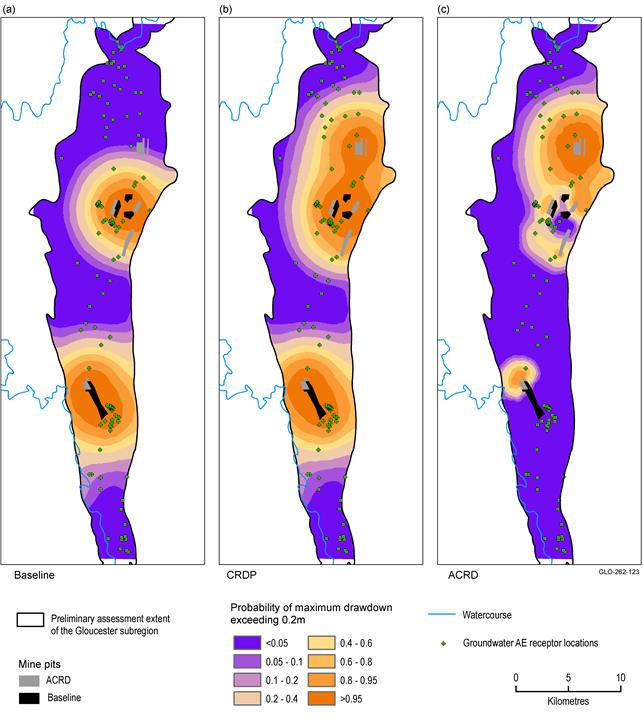
The 10,000 posterior parameter ensembles in Figure 34 are evaluated for each receptor location using the tailor-made emulator for that particular dmax or tmax prediction. A limited set of 200 parameter combinations, randomly selected from the posterior parameter ensembles is evaluated with the original model to compute dmax and tmax at the output nodes shown in Figure 19 (Section 2.6.2.7.2.1). This dataset is used to visualise the spatial variation in dmax and tmax illustrated in Figure 37 as the probability of drawdown exceeding 0.2 m. This threshold is the smallest of the drawdown thresholds defined in the aquifer interference policy and it corresponds to the threshold for impact on groundwater-dependent ecosystems.
Data: Bioregional Assessment Programme (Dataset 1)
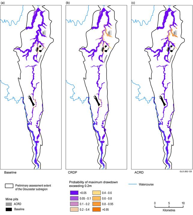
The map in Figure 37 shows the drawdown under baseline coal resource development (baseline) (a), under the coal resource development pathway (CDRP) conditions (b) and the difference between both, due to the additional coal resource development (c). The contour of a 5% probability of exceeding 0.2 m drawdown is situated slightly more than 5 km from the mine complexes. The effect of the lateral no-flow boundaries, representing the lateral boundary of the Gloucester geological basin, is clearly visible, especially to the east and west of the Duralie Coal Mine. The extent of the drawdown due to additional coal resource development is limited to the north of the Duralie Coal Mine, close to the planned extension. From Figure 37 (a) and (b), it is apparent that the majority of the drawdown of Duralie Coal Mine is realised under baseline conditions, where the extension to the north only results in minor drawdown due to additional coal resource development. A similar observation can be made for the Stratford Mining Complex. Central in the mine complex, the probability of the drawdown due to additional coal resource development exceeding 0.2 m is very small as most of the drawdown is realised under baseline conditions. The proposed Rocky Hill Coal Mine results in the largest area with high probability of drawdowns exceeding 0.2 m as there is no development under baseline conditions. There are no clear spatial patterns in drawdown that can be associated with CSG development.
Additional drawdown is the maximum difference in drawdown (dmax) between the coal resource development pathway (CRDP) and baseline, due to additional coal resource development
Data: Bioregional Assessment Programme (Dataset 1)
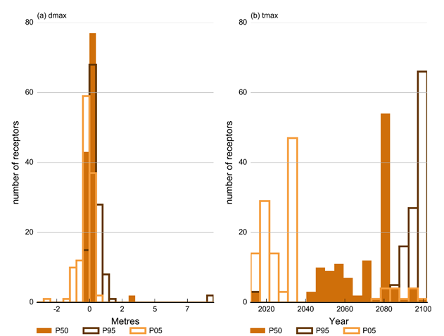
Figure 38 shows histograms of selected percentiles of the ensemble of dmax and tmax predictions at the receptor locations of the GW AEM. The most striking feature of this plot is that for the majority of receptors the median of the ensemble of drawdowns due to additional coal resource development is between –0.2 and 0.2 m. Only three receptors have a dmax value in excess of a meter. These are the three receptors in the immediate vicinity of the proposed Rocky Hill Coal Mine (Figure 37). At these locations the 95th percentile of dmax is close to 10 m. For some of the receptors situated in the close vicinity of the south-east corner of the Duralie Coal Mine, the 5th percentile of drawdown due to additional coal resource development can be as small as –1 m. This indicates that the GW AEM simulates a recovery of groundwater levels by 1 m as a result of the northwards extension of the mine (see Figure 20, Section 2.6.2.7.2.1).
The variation in year of maximum change due to additional coal resource development is much more variable, although for the majority of receptors the maximum change is only realised after 2040, after the planned coal mining and CSG operations in the Gloucester subregion have ceased.
dmax = maximum difference in drawdown
Data: Bioregional Assessment Programme (Dataset 1)
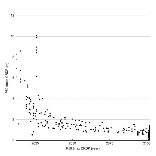
Figure 39 shows a scatterplot of the median predicted year of maximum change against the median predicted drawdown under coal resource development pathway at the analytic element output nodes. It is clear that drawdown decreases with time, that is, the largest drawdowns are realised the earliest and the drawdowns that occur towards the end of the simulation period are smaller than those that occur sooner.
Alluvial MODFLOW models
The posterior parameter ensembles of the alluvial MODFLOW models are combined with the posterior parameter ensemble of the analytic element model as the sensitivity analysis of the alluvial MODFLOW models highlighted that some of the analytic element parameters can affect the alluvial MODFLOW dmax and tmax predictions.
To generate the predictive ensembles at the receptor locations, the 10,000 parameter combinations are evaluated through the relevant emulators. A smaller set of 200 randomly selected parameter combinations from the posterior parameter ensembles, is evaluated with the original model to visualise the spatial patterns of drawdown shown in Figure 40.
The map in Figure 40 shows the drawdown under baseline conditions (a), under the CRDP conditions (b) and the difference between both, due to the additional coal resource development (c). The extent of the hydrological change is less than in the surface weathered and fractured rock layer. Probabilities of exceeding 0.2 m drawdown are limited to the immediate vicinity of the mine complexes. Drawdown due to additional coal resource development in excess of 0.2 m is only predicted to occur in the alluvium west and south of the proposed Rocky Hill Coal Mine. In the vicinity of the Stratford Mining Complex and Duralie Coal Mine, the probability of drawdown due to additional coal resource development exceeding 0.2 m is generally less than 5%.
It is noteworthy that underneath the rivers or, more correctly, the grid cells assigned a drain boundary condition, the probability of drawdown is very small. Only in the alluvium south of the proposed Rocky Hill Coal Mine and the alluvium flanked by the Stratford Mining Complex development are drawdowns in excess of 0.2 m predicted. This is not predicted to occur in the alluvium in the vicinity of the Duralie Coal Mine.
Maximum drawdown refers to the maximum difference in drawdown (dmax) for one realisation within an ensemble of groundwater modelling runs, obtained by choosing the maximum of the time series of differences between two futures.
The difference in drawdown between CRDP and baseline is due to the additional coal resource development (ACRD). Drawdown under the baseline is relative to drawdown with no coal resource development; likewise, drawdown under the CRDP is relative to drawdown with no coal resource development.
Data: Bioregional Assessment Programme (Dataset 2)
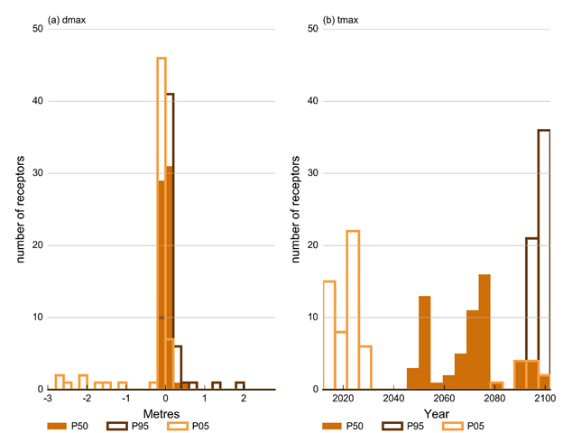
Additional drawdown is the maximum difference in drawdown (dmax) between the coal resource development pathway (CRDP) and baseline, due to additional coal resource development (ACRD).
tmax = year of maximum change
Data: Bioregional Assessment Programme (Dataset 2)
The histograms of drawdown due to additional coal resource development and year of maximum change at the alluvial MODFLOW model receptor locations are shown in Figure 41. The median predicted values of drawdown due to additional coal resource development values are between –0.2 m and 0.6 m. For more than 90% of the receptors, the drawdown due to additional coal resource development is between –0.2 m and 0.2 m. Receptors in the vicinity of Duralie Coal Mine (Figure 10, Section 2.6.2.3.3.2) are predicted to recover, with the 5th percentile of dmax at some locations smaller than –2.5 m. Receptors close to the proposed Rocky Hill Coal Mine are simulated to have the 95th percentile of dmax in excess of 1.5 m.
The median values of the year of maximum change due to additional coal resource development are very similar to those of the analytic element model, ranging from 2040 to 2100, beyond the time water extraction for coal resource development in the region is planned to cease. The 5th percentile of tmax does indicate that it is possible for drawdown due to additional coal resource development to be achieved during the active water extraction. This occurs at receptor locations close to mine footprints. Receptors further away from the mine footprints experience the drawdown at the end of or beyond the simulation period. As shown in submethodology M07 (as listed in Table 1) for groundwater modelling (Crosbie et al., 2016) and Figure 39, dmax realised at large tmax are smaller than dmax realised at earlier times.
2.6.2.8.1.4 Comparison with existing models
Section 2.6.2.2 provides a review of the development and results of previous modelling projects in the subregion. A direct comparison between these model results and the predictions provided in this study is not straightforward. The existing models are all deterministic (i.e. they provide a single estimate of hydrological change based on a single parameter combination that is considered optimal), while the bioregional assessment (BA) provides probabilistic ensembles of predictions, based on a range of likely parameter combinations. The BA models have selected the drawdown due to additional coal resource development as the primary prediction, where most regional models only provide outputs at selected times in the future. A final factor complicating a direct comparison is the difference in conceptualisation, boundary conditions and, most importantly, the implementation of coal resource development.
The models reviewed in Section 2.6.2.2 all predict negligible drawdowns at existing production bores. This is in line with the findings in this study, where the median of the drawdown due to additional coal resource development at the receptors, which include the production bores, is close to zero (Figure 38 and Figure 41).
The probabilistic modelling presented in this product does indicate that there is a 5% probability to exceed 0.2 m drawdown up to about 5 km from the mine footprint in the surface weathered and fractured rock layer. This is comparable with the estimate for the Stratford Mining Complex modelling, where 1 m of drawdown was predicted at the end of mining (December 2024) out 1 km around all pits, except south of Roseville West Pit where it may extend to 1.6 km. The Stratford Mining Complex modelling included a scenario in which coal seams in AGL’s Stage 1 gas field development area are dewatered to represent the cumulative impact of CSG extraction and coal mining. In this scenario very large drawdowns are realised in the surface weathered and fractured rock layer. The corresponding pumping rates are, however, not reported and it is therefore not possible to judge if the water production rates from CSG production are in the same order of magnitude of the water production rates simulated by AGL or used in the modelling presented in this product.
The modelling reports for the proposed Rocky Hill Coal Mine and Duralie Coal Mine did not provide estimates of drawdown in the surface weathered and fractured rock layer amenable for comparison with the BA modelling.
The surface water network in the Stratford Mining Complex, proposed Rocky Hill Coal Mine and Duralie Coal Mine groundwater models is represented using the RIVER package in MODFLOW. As outlined previously, this allows for drawdown to be compensated by influx of water through the river bed. These groundwater models therefore predict very limited drawdown in the alluvium, while the BA models indicate that there is a probability of exceeding 0.2 m drawdown in alluvial systems in the immediate vicinity of mines.
As mentioned in Section 2.6.2.1 and Section 2.6.2.7, the components of the water balance are reported in companion product 2.5 for the Gloucester subregion (Herron et al., 2018, Table 6, Table 7 and Table 8).
Product Finalisation date
- 2.6.2.1 Methods
- 2.6.2.2 Review of existing models
- 2.6.2.3 Model development
- 2.6.2.4 Boundary and initial conditions
- 2.6.2.5 Implementation of coal resource development pathway
- 2.6.2.6 Parameterisation
- 2.6.2.7 Observations and predictions
- 2.6.2.8 Uncertainty analysis
- 2.6.2.9 Limitations and conclusions
- Citation
- Acknowledgements
- Currency of scientific results
- Contributors to the Technical Programme
- About this technical product

