In the design of experiment phase of the uncertainty analysis workflow (Figure 6, Section 2.6.2.1) a set of parameter combinations and corresponding model outputs is generated by evaluating the GW AEM and the alluvial MODFLOW models a large number of times, to train the emulators that replace the model chain in the uncertainty analysis. This training dataset is also used for the formal sensitivity analysis. Ten thousand different combinations are generated of the parameters of the GW AEM (listed in Table 5 of Section 2.6.2.6.1), the alluvial MODFLOW models (listed in Table 6 of Section 2.6.2.6.2) and the AWRA-L model (listed in Table 7 of Section 2.6.1.5.1 in companion product 2.6.1 for the Gloucester subregion (Zhang et al., 2018)).
The number of samples is considered sufficient if, emulators trained with that number of samples are able to accurately predict the model response for unsampled parameter combinations (Sacks et al., 1989). Due to the large number of predictions that are required from the model chain, it is not possible to guarantee that the sampling scheme is sufficient for each and every individual prediction. The accuracy of the emulators is, however, individually evaluated and emulators that do not satisfy the accuracy criteria are omitted from the uncertainty analysis (see Section 2.6.2.7.4).
A pragmatic choice is made to generate 10,000 parameter combinations of the entire model chain in the design of experiment. The size of the training set, 10,000 samples, is a trade-off between the sampling density of parameter space and computational resources available (both in run-time and storage space). The bioregional assessment (BA) modelling team used the Pearcey and Bragg clusters, which are part of the High Performance Computing facilities of CSIRO (CSIRO, 2016) to evaluate the model runs for the design of experiment and the subsequent training and running of the emulators for the uncertainty analysis.
The design of experiment set of parameter combinations is generated using a maximin Latin Hypercube design (see Santner et al., 2003, p. 138). Latin Hypercube sampling is a stratified random sampling of a multivariate parameter space designed to provide an even coverage of parameter space (Iman, 2008). The maximin Latin Hypercube design is generated like a standard Latin Hypercube design, one design point at a time, but with each new point selected to maximise the minimum Euclidean distance between design points in the parameter space. Points in the design span the full range of parameter values in each dimension of the parameter space, but also avoid redundancy among points by ensuring that no two samples are too close together (since nearby points are likely to have similar model output).
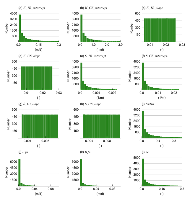
Figure 21 shows histograms of the 10,000 parameter combinations. The parameters are sampled uniformly on a log10 scale (K_IB_intercept, K_CS _intercept, S_IB_intercept, S_CS_intercept, KvKh, Kfh, Kfv, ne) or on a natural scale (K_IB_slope, K_CS_slope, S_IB_slope, S_CS_slope). In the design of experiment, no correlation between parameters is specified.
2.6.2.7.3.1 Analytic element model
Refer to Table 5 in Section 2.6.2.6.1 for definitions of terms.
Data: Bioregional Assessment Programme (Dataset 1)
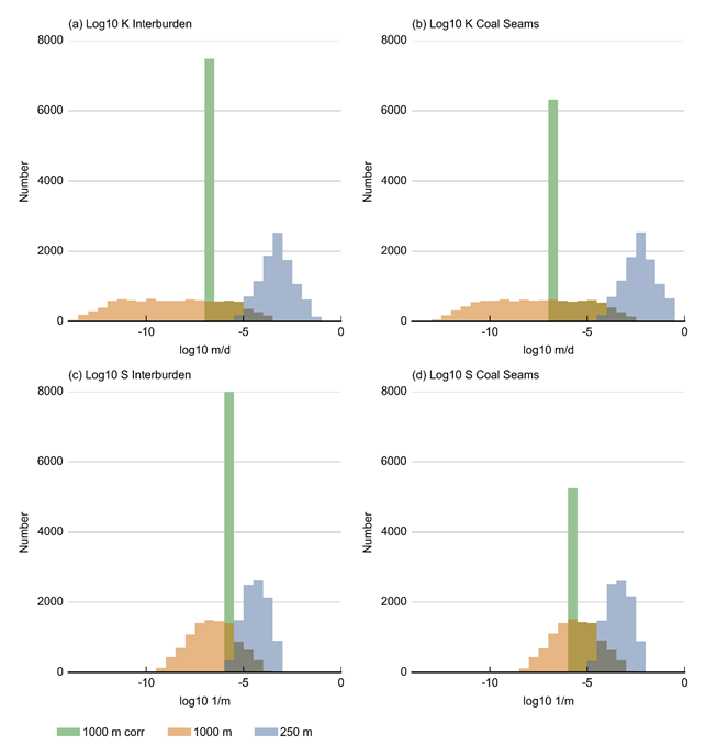
Figure 22 shows the actual hydraulic conductivities and storage assigned to the model based on this Latin Hypercube sampling for two nominal depths: 250 m and 1000 m. As mentioned in Section 2.6.2.6, the numerical model implements lower threshold values to ensure numerical stability. These are also incorporated in Figure 22.
1000 m corr incorporates the lower threshold of 1 x 10⁻⁷ m/day for hydraulic conductivity and 1 x 10⁻⁶ for storage
Data: Bioregional Assessment Programme (Dataset 1)
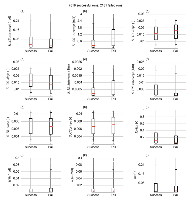
Ten thousand parameter combinations are evaluated, 7819 of these simulations produced dmax and tmax values; 2181 returned a ‘Not a Number’ value for at least one receptor. These failed runs represent parameter combinations for which the GW AEM could not arrive at a converging solution. Figure 23 shows box and whisker plots of the parameter ranges that gave rise to successful and failed model runs. In these plots, the box represents the interquartile range (25th to 75th percentile) and the whiskers extend from the 5th to the 95th percentile. The median is indicated by a horizontal line through the interquartile box. Outliers, points below the 5th percentile or above the 95th percentile, are depicted as black points.
Failed model runs appear to be limited for parameter combinations that lead to low vertical conductivity of the interburden (low K_IB_intercept, high K_IB_slope and low KvKh) and high interburden storage (high S_IB_intercept) in combination with elevated hydraulic conductivity/low storage of the coal seams (high K_CS_intercept, low K_CS_slope, low S_CS_intercept).
These parameter combinations result in a fast and large drawdown in the coal seam, which cannot be replenished quickly enough through the interburden because of its low Kv. The pumping rate required to maintain the prescribed head in the CSG wells becomes increasingly small, which gives rise to numerical precision errors that in turn result in ‘Not a Number’ values for the CSG pumping rate. CSG pumping is implemented as a two-stage process (see Section 2.6.2.5). Pumping rate is computed in the first stage from a prescribed head boundary condition that will be implemented in a second stage as a prescribed flux.
In the failed runs, the prescribed flux is not available and hence the CRDP run fails. A case can be made to assign a zero-prescribed CSG pumping rate to the failed runs and run these again to at least simulate the cumulative impact of coal mining in the weathered zone for these parameter combinations. Another option is to limit the range of the parameters in the sensitivity analysis run, to ensure failed runs do not occur. As both options represent a manipulation of the model runs, these options are not implemented and in the further analysis, the failed model runs are omitted. The information from the failed runs will, however, be incorporated in specifying the prior distributions of the parameters and their covariance for the uncertainty analysis (Section 2.6.2.8).
A failed run is a run which returned a ‘Not a Number’ value for dmax and tmax for at least one receptor. Refer to Table 5 in Section 2.6.2.6.1 for definitions of terms.
Data: Bioregional Assessment Programme (Dataset 1)
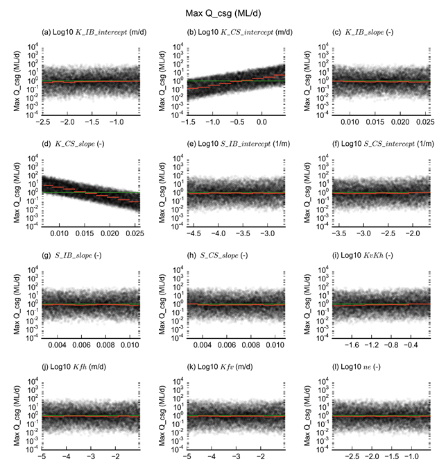
Each dot represents a single simulation. The red lines show the median value of dmax over the parameter range spanned by the line. The green line is the maximum water production rate threshold of 1.1 ML/day based on AGL Energy Limited (2015) predicted water extraction rates. Refer to Table 5 in Section 2.6.2.6.1 for definitions of terms.
Data: Bioregional Assessment Programme (Dataset 1)
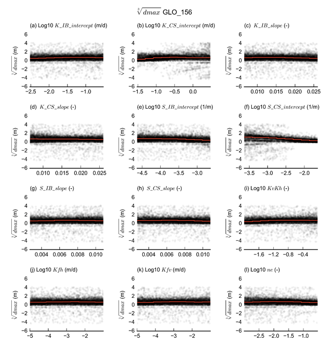
The values of dmax and tmax are discussed in depth in Section 2.6.2.8, when the final posterior distributions of the dmax and tmax for each receptor are available. To gain a better understanding of model behaviour, however, the effect of the parameters on the maximum CSG production rate (Figure 24) and on the dmax values for receptor GLO_156, 2 km north from the Stratford Mining Complex and 2 km south of the Rocky Hill Coal Project (Figure 25), are examined. Rather than plotting the dmax values directly, they are transformed by taking the cubed root. This transformation increases the resolution for both positive and negative values.
From Figure 24 it is apparent that the maximum CSG production rate is controlled by the hydraulic conductivity of the coal seams (K_CS_intercept and K_CS_slope). The log of the maximum water production rate increases linearly with increasing hydraulic conductivity. An increase in the intercept of the exponential decrease function leads to higher conductivity values at depth. A decrease in the slope of equation 6 in Section 2.6.2.6 will have the same effect, higher conductivity at depth.
Almost half of the parameter combinations of the design of experiment result in maximum CSG water production rates in excess of 1.1 ML/day, the threshold value above which maximum water production rates are considered unrealistically high (see Section 2.6.2.7.1). This indicates that a sizeable proportion of the wide parameter range sampled in the design of experiment (Figure 25 and Figure 22) gives rise to unrealistically high CSG water production rates. Section 2.6.2.8 describes how the parameter range is constrained in the uncertainty analysis to avoid these unrealistic parameter combinations in the posterior parameter ensemble that is used to generate the posterior prediction ensemble.
Figure 25 shows the variation of the maximum difference in drawdown, dmax, in function of the parameter values of the design of experiment. One of the most striking features in Figure 25 is the presence of negative dmax values. These values appear to be limited to parameter combinations with high K_CS_Intercept and low S_CS_intercept values. These extreme and unlikely parameter combinations cause numerical instabilities which result in failed runs or negative drawdown due to additional coal resource development. The numerical instability occurs because the large fluxes generated by high hydraulic conductivity result in extremely high hydraulic gradients due to the low storage.
The red lines are the median of dmax in the parameter range spanned by the line. For this particular receptor, GLO_156, it is apparent that the two most influential parameters are S_CS_intercept and K_CS_intercept.
The intercept of the depth–S relationship for the coal seam, S_CS_intercept, shows a marked response in which drawdown increases with decreasing storage. This is likely an effect limited to the weathered zone, where, per definition of storage, for a volume of water extracted from an aquifer, small storage values result in large drawdowns and large storage values result in small drawdowns.
Decreasing the intercept of the depth–K relationship for the coal seam, K_CS_intercept, decreases both the K of the weathered zone and the K of the coal seams. A decrease of hydraulic conductivity in the weathered zone has a result that the cone of depression becomes deeper, as the resistance is higher for water to flow laterally to replenish the water extracted by the mines.
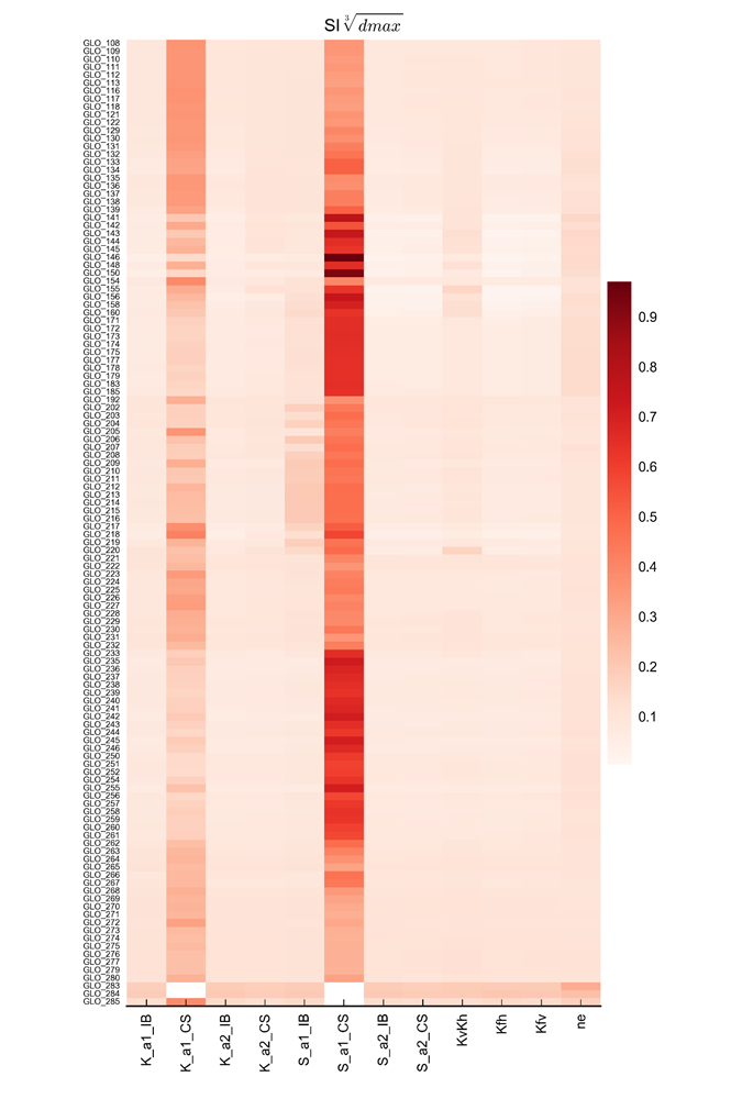
A detailed discussion for each receptor of these relationships is beyond the scope of the report. Figure 26 does show the sensitivity index of the cube root of dmax for each parameter–receptor combination, calculated with the density-based sensitivity index introduced by Plischke et al. (2013). Larger values of the sensitivity index indicate higher sensitivity of the prediction to the parameter. The cube root transform is chosen to compensate for the skewed distribution of most of the dmax values. It is apparent that the K and S intercept of the coal seams (and thus the weathered zone) are the dominant factors for most receptors.
Each dot represents a single simulation. The red lines show the median value of dmax over the parameter range spanned by the line. Refer to Table 5 in Section 2.6.2.6.1 for definitions of terms.
Data: Bioregional Assessment Programme (Dataset 1)
Larger values indicate higher sensitivity of a receptor to a parameter. Refer to Table 5 in Section 2.6.2.6.1 for definitions of terms.
Data: Bioregional Assessment Programme (Dataset 1)
2.6.2.7.3.2 Alluvial MODFLOW models
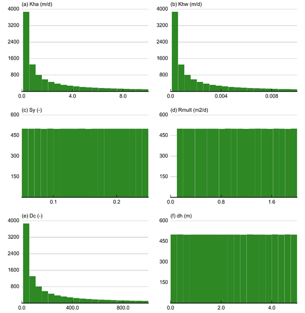
In the design of experiment of the sensitivity analysis of the Gloucester model chain, 10,000 parameter combinations of the MODFLOW Avon and Karuah models are generated and evaluated for both models. Figure 27 shows histograms of the parameter values in the design of experiment. The hydraulic conductivity of the weathered zone (Khw) and the alluvium (Kha) and the drainbed conductance are uniformly sampled in log10 space while the other parameters, the specific yield (Sy), the recharge multiplier (Rmult) and the constant head offset (dh) are uniformly sampled in native space.
(a) Saturated hydraulic conductivity of top alluvial layer (Kha (m/day)); (b) Saturated hydraulic conductivity of lower weathered layer (Khw (m/day)); (c) Specific yield of the top alluvial layer (Sy (-)); (d) Hydraulic conductance of lower boundary of drain bed (Dc (m2/day); (e) Multiplier for monthly recharge (Rmult (-)); and (f) Depth to water in the lower weathered layer (dh (m)). Refer to Table 5 in Section 2.6.2.6.1 for definitions of terms.
Data: Bioregional Assessment Programme (Dataset 5)
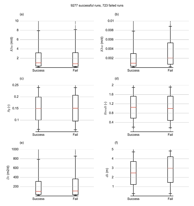
From the 10,000 runs, 723 failed to converge. Figure 28 shows that failed model runs are associated with high hydraulic conductivity values for the alluvium (Kha) and a low specific yield (Sy). This physically unrealistic combination of parameters allows for the alluvial layer to drain too quickly and become dry. This causes numerical instability preventing the model to converge.
(a) Saturated hydraulic conductivity of top alluvial layer (Kha (m/day)); (b) Saturated hydraulic conductivity of lower weathered layer (Khw (m/day)); (c) Specific yield of the top alluvial layer (Sy (-)); (d) Hydraulic conductance of lower boundary of drain bed (Dc (m2/day); (e) Multiplier for monthly recharge (Rmult (-)); and (f) Depth to water in the lower weathered layer (dh (m)). Refer to Table 5 in Section 2.6.2.6.1 for definitions of terms.
Data: Bioregional Assessment Programme (Dataset 5)
Qdr = drainage flux; Qup = alluvium – weathered zone exchange flux
Data: Bioregional Assessment Programme (Dataset 5)
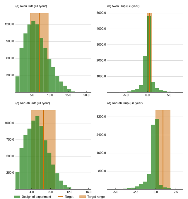
Figure 29 shows histograms of the simulated drainage fluxes and upward fluxes into the alluvium for the Avon and Karuah models, compared to their target range from Table 7. The simulated drainage fluxes are close to the target distributions, while the current range of parameters evaluated in the design of experiment appears to underestimate the upward flux, especially for the Karuah model. During the uncertainty analysis, a Markov chain Monte Carlo simulation is carried out to select parameter combinations that are in agreement with the target distributions.
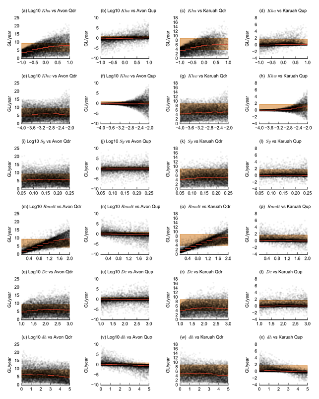
Figure 30 shows the response of the drainage and upward fluxes to variations in parameter values for the Avon and Karuah models.
The drainage flux in both Avon and Karuah models is controlled by the hydraulic conductivity of the alluvium and the recharge multiplier, where increases in these parameters lead to increases in drainage flux. The other parameters do affect the drainage flux, but to a much lesser extent.
The magnitude of the upward flux is completely dominated by the hydraulic conductivity of the weathered zone. The direction of flow appears to be controlled primarily by the offset of the specified head boundary condition. Secondary controlling factors are the hydraulic conductivity of the alluvium and the recharge multiplier. The upward flux is a function of the hydraulic gradient between the alluvium and the weathered zone. Large dh values result in fluxes towards the weathered zone. Elevated groundwater levels in the alluvium, through low Kha or high Rmult, will also result in fluxes towards the weathered zone.
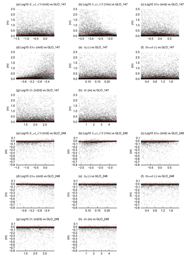
Figure 31 illustrates the response of drawdown due to additional coal resource development at the receptor locations to variations in parameter values for two representative receptors: GLO_147 in the Avon model and GLO_248 in the Karuah model. These plots include the two parameters that control drawdown in the weathered zone from the regional model, namely K_CS_intercept and S_CS_intercept.
For both receptors it is clear that the most important parameter is the hydraulic conductivity in the weathered zone (Khw), followed by the weathered zone parameters of the regional model. The hydraulic conductivity and storage in the alluvium are of lesser importance, as is the recharge multiplier and drainbed conductance and constant head offset. This indicates that the drawdown due to additional coal resource development is dominated by the magnitude of the change in flux at the bottom of the alluvium.
The red lines indicate the median y-axis value over the range spanned by the width of the line. The orange band indicates the target range of the y-axis. Qdr = drainage flux; Qup = alluvium – weathered zone exchange flux. Refer to Table 5 in Section 2.6.2.6.1 for definitions of terms.
Data: Bioregional Assessment Programme (Dataset 5)
Refer to Table 5 in Section 2.6.2.6.1 for definitions of terms.
Data: Bioregional Assessment Programme (Dataset 5)
In Figure 32 this sensitivity is quantified for all dmax parameter–receptor combinations with the density-based sensitivity index introduced by Plischke et al. (2013). Rows in the figure without colour coding indicate receptors with an impact too small to analyse. The sensitivity indices confirm that, in general terms, S_CS_intercept, K_CS_intercept and Khw dominate the magnitude of dmax for most receptors. Note that the water balance targets are not able to greatly constrain these parameters.
Product Finalisation date
- 2.6.2.1 Methods
- 2.6.2.2 Review of existing models
- 2.6.2.3 Model development
- 2.6.2.4 Boundary and initial conditions
- 2.6.2.5 Implementation of coal resource development pathway
- 2.6.2.6 Parameterisation
- 2.6.2.7 Observations and predictions
- 2.6.2.8 Uncertainty analysis
- 2.6.2.9 Limitations and conclusions
- Citation
- Acknowledgements
- Currency of scientific results
- Contributors to the Technical Programme
- About this technical product

