2.6.2.3.5.1 Analytic element model
The model layers are horizontal, of constant thickness and infinite in extent. The top of the model is set at an arbitrary level of zero metres and the total thickness of the simulated sedimentary column is less than 1000 m.
The groundwater system is implemented as an alternating sequence of aquifers and aquitards (Figure 8). Groundwater level and flow are only simulated for the aquifers. The flow between two successive aquifers is controlled by the hydraulic gradient between them and the hydraulic properties assigned to the aquitard separating both aquifers. In this model, the starting aquifer is the weathered zone with a nominal thickness of 75 m (McVicar et al., 2014). Deeper down in the basin, only the coal seams are considered to act as aquifers. The interburden is simulated as aquitards. This implies that no groundwater levels in the aquitards are calculated.
The coal seams are assigned a nominal thickness of 3 m each, in accordance with the coal seam thickness reported in companion product 1.1 for the Gloucester subregion (McVicar et al., 2014, Figure 24). The number and position of the coal seams are generated stochastically, allowing for the density of coal seams to vary with depth, according to stratigraphy (see McVicar et al., 2014, Figure 24). Coal seams are considered to be between 250 and 1000 m in depth. In reality, coal seams are present outside this range, but CSG exploitation will only occur within this depth range (see companion product 1.2 for the Gloucester subregion (Hodgkinson et al., 2014, Section 1.2.3.2, p. 26)). An example of a single stochastic realisation of the distribution of coal seams is shown in Figure 11.
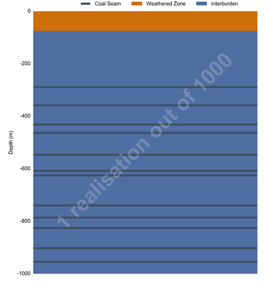
Figure 11 Single realisation of coal seam distribution for the Gloucester subregion
Data: Bioregional Assessment Programme (Dataset 3)
As stated in companion product 1.1 for the Gloucester subregion (McVicar et al., 2014, Section 1.1.3.1.1), throughout all of the Permian strata, normal, strike-slip and reverse faults occur. The fault density is higher near the flanks and faults orientations are generally northerly striking with dips toward the central axis of the geological basin. Major fault trends are implemented as linear features that provide a vertical connection between all layers and a horizontal impedance to flow. The flow rate through the major faults is controlled by the fault hydraulic conductivity. The position of the major fault trends is inferred from geological maps and geological modelling from companion product 2.1-2.2 for the Gloucester subregion (Frery et al., 2018). Note that in this interpretation of the structural features of the Gloucester Basin, fewer faults are identified compared to those identified on the geological map of the region (Roberts et al., 1991). Figure 12 shows the position and probability of the major fault trends. The geographic location of the potential major faults is considered known and kept fixed for all realisations, whereas their probability of occurrence at those locations is treated as a stochastic process. In other words, every realisation can be different in terms of presence or absence of major faults.
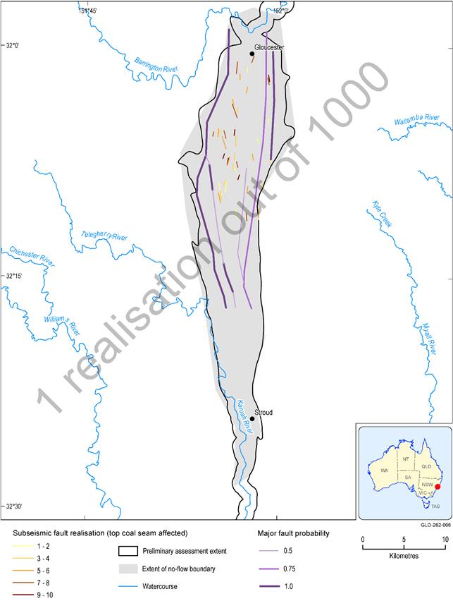
Data: Bioregional Assessment Programme (Dataset 3)
Subseismic faults, which are faults with a displacement too small to be identified from a seismic section, less than 100 m, are generated stochastically in the vicinity of the planned coal resource development. For the GW AEM, the subseismic faults of interest are those with a fault height between 200 and 1000 m, where the fault height is the vertical extent of the fault zone. Larger faults can be identified on seismic sections and are assumed to be mapped at the regional scale as part of the major fault network. Faults with heights less than 200 m are not considered to be important for the regional groundwater model as it is unlikely that these faults are large enough to alter regional groundwater flow.
Fault heights are, however, very hard to measure. A more common and less ambiguous measure to characterise faults is the fault displacement. Figure 13 in Section 2.1.2.2 in companion product 2.1-2.2 (Frery et al., 2018) shows a number of type curves for the Gloucester subregion to relate fault displacement and cumulative number of faults. These type curves can be used to estimate the number of faults with a given displacement. The displacement range that corresponds to the fault height range of interest (between 200 and 1000 m) is based on a number of global datasets. Nicol et al. (1996) estimated the average ratio between fault height (H) and fault length (L) (the length of a fault along strike) to be equal to 2.15. The fault height range of 200 to 1000 m corresponds to approximate fault lengths of 400 to 2000 m. On a similar dataset, Kim and Sanderson (2005) empirically established a ratio of 0.01 between maximal displacement or throw and fault length. Faults between 400 and 2000 m then correspond to a throw range between 4 and 20 m. For that throw range, in a 10 x 10 km area (the scale that corresponds most closely to the size of the Gloucester Basin), the fault length distribution (X) in the Gloucester subregion can be approximated by taking 40 samples from a beta distribution (Bailey et al., 2005; Frery et al., 2018):
|
|
(5) |
The strike of the faults is chosen to align with the major tectonic axis of the basin and to vary between 338° and 022°.
One thousand stochastic realisations of the subseismic fault network are generated, each comprising 40 faults that connect three model aquifers (coal seams or surface weathered and fractured rock layer) with each other. Determining which model aquifers are connected is also part of the stochastic process. Figure 12 shows a single realisation of a subseismic fault network. The number of realisations proved to be sufficient to ensure that the entire region was represented as faulted.
The generation of subseismic faults is limited in extent. The north and south limits were chosen at a distance beyond the proposed CSG development area. Any subseismic faults outside this domain are considered to have a negligible effect on the predictions.
The generation of a stochastic network was done in the following steps:
- Take 40 samples from the beta distribution to get the fault lengths.
- Take 40 random uniform samples of an angle between 338° and 022°.
- In a ‘for’ loop:
- generate a random point within the extent of the subseismic fault domain as the starting point for a fault
- calculate the endpoint of the fault from the fault length vector and angle vector
- accept the fault if it is fully contained within the domain, otherwise reject it and go back to step a.
- Assign random upper coal seam a number between one and ten, add two to obtain lower coal seam.
The watertable is situated in the surface weathered and fractured rock layer (Figure 8). To represent the phreatic part of this weathered zone, a leaky layer is simulated on top of the sequence of aquitards and aquifers, in line with the recommendation in Hemker (1985). Groundwater levels are not computed in this layer, but it allows the simulation of the release of water from storage due to dewatering of the phreatic part of the weathered zone.
2.6.2.3.5.2 Alluvial MODFLOW models
The geometry of the active area is controlled by the mapped extent of alluvium and the DEM (Farr et al., 2007). The alluvial layer is fixed to be 15 m thick and exactly follows the topography, while the second layer extends down to an arbitrary datum.
No aquitards exist in the vertical model domain, only a vertical hydraulic conductivity between the two layers to control flow between them based on head difference.
The fault network in the analytic element model is not propagated in the alluvium as there is no indication to date that hydraulic properties in the alluvium are affected by fault activity. It is trivial, however, to change the hydraulic properties of the alluvial models locally should future observations indicate fault activity has altered hydraulic conductivity in the alluvium.
