As outlined in Section 2.6.2.1, the groundwater model is evaluated for a wide range of parameter combinations chosen in a systematic and efficient way that we refer to as the design of experiment (see companion submethodology M09 (as listed in Table 1) for propagating uncertainty through models (Peeters et al., 2016)). The results of these model runs, the simulated equivalents to the observations described in Section 2.6.2.7.1 and the predictions described in Section 2.6.2.7.2, are used to train statistical emulators, which replace the original model in the uncertainty analysis. Each parameter is sampled across a wide range to ensure sufficient coverage of the parameter space. The design of experiment model runs also allow a comprehensive sensitivity analysis to be undertaken. Such an analysis provides insight into the functioning of the model and aids in identifying which parameters the predictions are most sensitive to and if the observations are able to constrain these parameters.
Table 8 lists the ten parameters that were varied in the sensitivity and uncertainty analysis and how they relate to the hydraulic properties, stresses and boundary conditions of the groundwater model. The ‘Section’ column provides the section number in this product where the parameter is discussed, while the ‘Notes’ column provides more detail on the implementation of the parameters. The ‘Min’ and ‘Max’ columns provide the range over which the parameter is sampled. Not all the model parameters were carried through to the uncertainty analysis. Rationalising the number of parameters was undertaken to reduce the total number of simulations needed to characterise modelling uncertainty. Where a number of parameters are used to define a process in the model, it is possible to fix some and vary others to obtain a satisfactory characterisation of the range of possible outcomes. The use of multipliers, such as ne, Kh and K_ramp, ensures that all model parameters related to the hydraulic properties in the model are varied systematically during the uncertainty analysis. The unsaturated-flow parameters and the river stage height are not varied in the uncertainty analysis as their effect on predictions is strongly correlated with other included parameters. For example, the effect on predictions of varying river stage height can largely be determined through varying riverbed depth addition. Likewise, changes in unsaturated-flow properties are linked to the saturated-flow properties, which means the uncertainty in the unsaturated-flow properties is reflected in the uncertainty of the saturated-flow properties. The general-head conductance and depth control on evapotranspiration are not included in the uncertainty analysis as initial model runs indicated that these parameters have a very limited effect on predictions. This is explored for evapotranspiration-extinction depth in more detail in Section 2.6.2.8.2.16.
Table 8 Parameters included in the sensitivity and uncertainty analysis
|
Parameter |
Description |
Section |
Min |
Max |
Notes |
|---|---|---|---|---|---|
|
Q_mine |
Mine water extraction multiplier |
2.6.2.5 |
0.5 |
1.5 |
All groundwater extraction rates by mines are multiplied by this quantity. |
|
C_riv |
Riverbed conductance multiplier |
2.6.2.4 |
0.1 |
10 |
The riverbed conductance is multiplied by this quantity. |
|
d_riv |
Riverbed depth addition (m) |
2.6.2.4 |
–5 |
5 |
Depth of the river points defined as:
The depth of the river points thus varies from 0 to 10 m below topography. |
|
RCH |
Rainfall recharge multiplier |
2.6.2.4 |
0.5 |
1.5 |
Rainfall recharge is multiplied by this quantity. |
|
ne_lambda |
Decay parameter for porosity (ap) |
2.6.2.6 |
0.005 |
0.015 |
The baseline porosity is 0.1 for lithologies 1 to 6, and 0.2 for lithology 7. It is multiplied by the multiplier, and the exponential decay is used to find the porosity at a certain depth. However, porosity is constrained to be always greater than 0.0001 to ensure convergence of the numerical model. |
|
ne |
Baseline porosity multiplier |
2.6.2.6 |
0.3 |
3 |
|
|
K_lambda |
Decay parameter for horizontal and vertical conductivity (ah and av) |
2.6.2.6 |
0.01 |
0.04 |
The same exponential decay parameter is chosen for horizontal and vertical conductivity. The baseline horizontal conductivity is 0.5 m/day for lithologies 1 to 6, and 1 m/day for lithology 7. The baseline vertical conductivity is 0.05 m/day for lithologies 1 to 6, and 1 m/day for lithology 7. An upper bound of 100 m/day and a lower bound of 10-6 m/day is placed on all conductivities. See Section 2.1.3 in companion product 2.1-2.2 for the Hunter subregion (Herron et al., 2018) for a comparison with measured data. |
|
Kh |
Horizontal hydraulic conductivity multiplier |
2.6.2.6 |
0.1 |
10 |
|
|
KvKh |
Ratio Kv/Kh |
2.6.2.6 |
0.01 |
1 |
|
|
K_ramp |
Conductivity enhancement multiplier |
2.6.2.5 |
0.2 |
1 |
All parameters, M, m, Z and z introduced in Section 2.6.2.5.3 are multiplied by this quantity. |
Three thousand parameter combinations were generated for the entire parameter space for the model sequence (i.e. each parameter combination has parameter values for the groundwater and surface water models) using a maximin Latin Hypercube design (see Santner et al., 2003, p. 138). The maximin Latin Hypercube design is generated like a standard Latin Hypercube design, one design point at a time, but with each new point selected to maximise the minimum Euclidean distance between design points in the parameter space. Points in the design span the full range of parameter values in each dimension of the parameter space, but also avoid redundancy amongst points by maximising the Euclidean distance between two points (since nearby points are likely to have similar model output). The parameter ranges are sampled uniformly from their range.
Within the available time frame and with the available computational resources, the modelling team was able to evaluate 1500 parameter combinations. Although the coverage of a ten-dimensional parameter space is limited with 1500 simulations, visual inspection of the parameter combinations evaluated showed that there was adequate coverage of all parameters and no bias or gaps in the sampling of the parameter hyperspace.
Section 2.6.2.7.4 describes the development of the emulators with these model results. A part of developing the emulators is verifying that the sampling density is sufficient to train the emulators with an acceptable mismatch between simulated and emulated prediction values. The following sections describe the sensitivity of the observations and predictions to the ten parameters.
2.6.2.7.3.1 Simulated equivalents to observations from the design of experiment
The best appreciation of the relationship between a parameter and an observation or prediction is through the inspection of scatter plots. The large dimensionality of parameters, observations and predictions precludes this type of visualisation for all parameter–prediction combinations, so a select few scatterplots are provided as illustration. A comprehensive assessment of sensitivity is provided through sensitivity indices. These indices, computed using the methodology outlined in Plischke et al. (2013), are a density rather than variance-based quantification of the change in a prediction or observation due to a change in a parameter value. It is a relative metric in which large values indicate high sensitivity, whereas low values indicate low sensitivity.
Figure 28 shows how the predicted groundwater levels at observation bore GW080967 in November 2005 vary with parameter values. The sensitivity index for each parameter is also shown. The green line indicates the observed groundwater level.
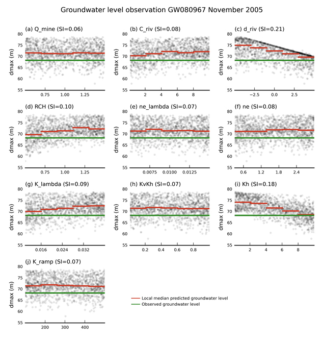
For each parameter, the corresponding sensitivity index (SI) is provided in the title. The sensitivity index is a relative metric in which high values indicate sensitive parameters and low values indicate less sensitive parameters. The red line indicates the local median of simulated values over the parameter ranges spanned by the line segment. The green line is the observed groundwater level.
dmax = maximum difference in drawdown between the coal resource development pathway (CRDP) and baseline, due to additional coal resource development (ACRD)
Data: Bioregional Assessment Programme (Dataset 2)
It is clear that a wide range of parameter values result in predicted groundwater levels matching the observed groundwater level at this location. However, only a few parameters noticeably affect the predicted groundwater levels:
- d_riv: the depth of river model nodes below topography where a d_riv equates to a depth below topography of 0 m and a d_riv of 5 m equals a depth of 10 m below topography
- Kh: the horizontal hydraulic conductivity multiplier
- RCH: the multiplier for spatially variable recharge
- K_lambda: the depth-decay parameter for horizontal and vertical hydraulic conductivity.
The depth below topography of the river model nodes controls the drainage level in the groundwater model and therefore imposes an upper boundary on the simulated groundwater levels, even at this observation location which is more than 15 km from the nearest river model node. For d_riv values less than 1 m, however, the parameter no longer controls groundwater levels. The hydraulic properties, Kh and K_lambda, both have a large influence. Higher hydraulic conductivities (high Kh and low K_lambda) result in lower simulated groundwater levels. The recharge multiplier, RCH, has a secondary effect, in which higher recharge values result in higher groundwater levels.
Figure 29a shows boxplots of the sensitivity indices for all available simulated equivalents to groundwater level observations. The same parameters identified as influential on the groundwater level at observation location GW080967 in November 2005 appear to be important for simulated equivalents at other groundwater level observation sites.
The simulated equivalents to groundwater level observations are not sensitive to Q_mine, C_riv, ne_lambda, ne and K_ramp. This is not surprising for Q_mine and K_ramp as they affect the mine pumping rates and hydraulic conductivity enhancement after longwall mine collapse, and will mostly affect future rather than historical simulated groundwater levels. The relative insensitivity of groundwater level predictions to the riverbed conductance (C_riv) and porosity (ne_lambda and ne) does not mean these variables have no effect, rather it indicates the effect of these parameters is small compared to other parameters and is too small to be distinguished based on a design of experiment with 1500 evaluated parameter combinations.
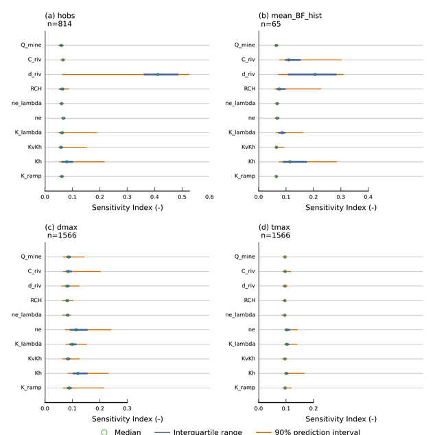
Data: Bioregional Assessment Programme (Dataset 2)
2.6.2.7.3.2 Simulated historical average surface water – groundwater flux
Figure 30 shows scatterplots of the parameter values versus the simulated average historical surface water – groundwater flux at gauge location 210083 for all of the evaluated design of experiment model runs. By far the most sensitive parameter is the depth of the river model nodes below topography (d_riv). The average historical baseflow increases almost linearly until the river model nodes are about 4 m below topography (d_riv equal to –1 m). For larger values of d_riv, however, the historical average baseflow remains almost constant and baseflow is positive. For positive baseflow values, the simulated baseflow appears to vary linearly with hydraulic properties (K_lambda and Kh), riverbed conductance (C_riv) and recharge (RCH). Figure 29b confirms that these parameters are influential for the other gauge locations as well.
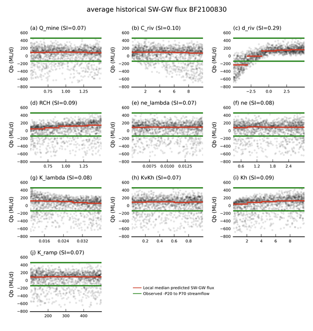
For each parameter, the corresponding sensitivity index (SI) is provided in the title. The sensitivity index is a relative metric in which high values indicate sensitive parameters and low values indicate less sensitive parameters. The red line indicates the local median of simulated values over the parameter ranges spanned by the line segment. The green lines indicate the observed negative of the 20th percentile and the 70th percentile.
Data: Bioregional Assessment Programme (Dataset 2)
2.6.2.7.3.3 Drawdown predictions (dmax) and year of maximum change (tmax)
Figure 31 shows scatterplots of the parameter values versus predicted maximum drawdown at model node probe_66 for all evaluated design of experiment model runs. The dominant parameter is Q_mine, the multiplier on the mine pumping rates. Increasing pumping rates lead to increases in drawdown. The hydraulic properties Kh and K_lambda are the next most important parameters. An increase in hydraulic conductivity (Kh increases and K_lambda decreases) leads to decreases in maximum drawdown. The K_ramp parameter, the enhancement of hydraulic conductivity after longwall mine collapse, shows a non-linear response, with the dmax values most sensitive for K_ramp values less than 200 m. The porosity parameters, ne and ne_lambda, have a small effect on the predicted drawdown, where increased porosity leads to smaller predicted drawdowns.
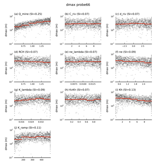
For each parameter, the corresponding sensitivity index (SI) is provided in the title. The sensitivity index is a relative metric in which high values indicate sensitive parameters and low values indicate less sensitive parameters. The red line indicates the local median of simulated values over the parameter ranges spanned by the line segment.
Data: Bioregional Assessment Programme (Dataset 2)
Figure 29c confirms these trends at the other model nodes, but provides a more nuanced understanding of the model behaviour. The two most important parameters across all model nodes are Kh and ne, followed by C_riv, K_ramp and Q_mine. The wide ranges in sensitivity index for some parameters reflect spatial variability in parameter sensitivity. For example, model nodes close to the river network are more sensitive to the riverbed conductance C_riv than model nodes away from the river network.
Figure 29d shows the sensitivity indices for the year of maximum change. Although the ranges of the sensitivity indices for ne, Kh and K_lambda are larger than for other parameters, there is no parameter that clearly dominates the year of maximum change. This indicates a large random component in this prediction as illustrated in Figure 24b and Figure 24d. A small change in either time series will have a negligible effect on the predicted drawdown, but can potentially drastically shift the year of maximum change.
