- Home
- Assessments
- Bioregional Assessment Program
- Hunter subregion
- 2.6.2 Groundwater numerical modelling for the Hunter subregion
- 2.6.2.4 Boundary and initial conditions
- 2.6.2.4.3 Surface water – groundwater interactions
2.6.2.4.3.1 Geometry
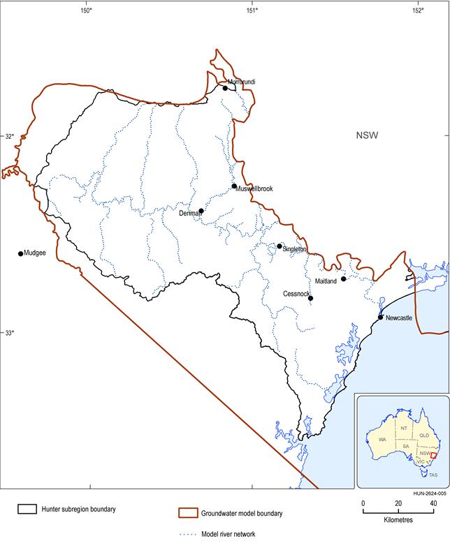
All major rivers (31 named reaches) within the Hunter subregion (Geoscience Australia, Dataset 8) are represented in the model. Some additional small reaches were added to ensure that change in baseflows could be generated along rivers represented in the AWRA-R (river) node-link network. The polylines used to define the locations of rivers in the groundwater model are shown in Figure 16.
Figure 16 River network for groundwater modelling
Data: Bioregional Assessment Programme (Dataset 9)
The Multiphysics Object-Oriented Simulation Environment (MOOSE) software used to implement and run the model cannot represent line sources and sinks, only point sources and sinks, so each river was decomposed into a sequence of points, spaced at 1 km intervals. This means baseflow is recorded only at 1 km intervals, rather than continuously along a river reach.
These points are placed at a depth of 5 m below the model’s topography. This is for two reasons. Firstly, rivers tend to incise channels below the land surface at a scale that may be too fine to be represented in the 3-second digital elevation model (Geoscience Australia, Dataset 2) used to define the surface topography. At some points on the river network, surveyed information has been recorded that could be used instead, but this is not available for most of the river network. Secondly, the model further discretises this digital elevation model with resolution as coarse as 15 km, so many points at their true elevation according to the digital elevation model would lie outside the model domain (above the model topography). For these two reasons it is appropriate to shift the points’ vertical position downwards. This shift is varied in the uncertainty analysis.
2.6.2.4.3.2 Baseflow and leakage
At each point, representing a 1 km section of river, along the river network, the model can lose water to represent fluxes to the river (i.e. baseflow) or gain water, representing leakage from the river, according to:
|
|
(3) |
|
|
|
(4) |
|
where:
- F is the flux out of the groundwater system (in kg/year) and is positive for baseflow and negative for leakage
- h is the groundwater level at the point
- h0 is the river stage height
- C is the riverbed conductance, which has a base value of 320 ML/m/year, but which is a parameter varied in the uncertainty analysis
- T is a parameter that limits the leakage. For perennial rivers T = –1 m, while for ephemeral rivers T = 0. This means there is no leakage for ephemeral rivers, while the leakage from perennial rivers does not increase once the water head is 1 m below h0.
The base value of C is motivated by assuming the riverbed has a width of order 10 m and thickness of order 1 m and conductivity of 0.1 m/day. The river stage height defaults to h0 = 3 m, for all points. However, because the depth of the points is varied in the uncertainty analysis, this effectively also varies h0.
2.6.2.4.3.3 AWRA-R baseflows
The surface water model contains 63 nodes at which the groundwater model can provide change in baseflow estimates. Nodes mostly correspond to streamflow gauging stations, but some nodes have been included specifically for assessing hydrological changes in response to coal resource development under the baseline and coal resource development pathway (CRDP). The baseflows (positive) and leakages (negative) are summed for all the points in the link upstream of a node in order to predict the total baseflow at the node. The numerical implementation of the groundwater model runs using nominal monthly time steps, so can only provide a monthly time series of gauge baseflows. The surface water model runs using daily time steps, and the groundwater results are interpolated linearly to provide this.

Product Finalisation date
- 2.6.2.1 Methods
- 2.6.2.2 Review of existing models
- 2.6.2.3 Model development
- 2.6.2.4 Boundary and initial conditions
- 2.6.2.5 Implementation of the coal resource development pathway
- 2.6.2.6 Parameterisation
- 2.6.2.7 Observations and predictions
- 2.6.2.8 Uncertainty analysis
- 2.6.2.9 Limitations and conclusions
- Citation
- Acknowledgements
- Currency of scientific results
- Contributors to the Technical Programme
- About this technical product

