2.1.2.2 Statistical analysis and interpolation

Observed datasets (Section 2.1.2.1) were processed to form derived datasets. These datasets were analysed and interpolated to develop a three-dimensional geological model at the basin scale. The three-dimensional geocellular model was built using RMS Roxar software. This package is commercial software developed by Emerson and used in the oil and gas industry. For more details, please refer to the RMS Roxar website (Emerson, 2016).

2.1.2.2.1 Workflow

A step by step workflow was designed to define the subsurface structural and stratigraphic architecture of the Gloucester Basin and support scientific reasoning through the data processing. It is based on classical 3D approaches (Ross et al., 2004) and adapted in order to produce a simple regional model from datasets that are poorly constrained. The aim of this workflow is to avoid inducing a structural complexity that is highly uncertain in the grid geometry (Wellmann et al., 2010).

This workflow comprised:

2.1.2.2.2 Data processing

Even if the data density is higher than in other subregions studied in the frame of the Bioregional Assessment Programme, the spatial distribution and density of the geological data in the Gloucester geological basin can be defined as poor: for instance, there is no large scale and good quality 3D seismic data and the wells are concentrated mainly in the Gloucester Gas Project area. For more details please refer to the companion product 1.1, the context statement for Gloucester subregion (McVicar et al., 2014).

Stratigraphic and structural information provided by the deep well dataset were processed to form the wells derived dataset. Well completion reports from the 24 selected deep wells (see the listing of well completion reports within the list of references following Section 2.1.2.3.) were analysed to determine each formation top depth (Table 4). The markers of the formation top depths in the wells are called ‘well picks’. The error in the formation top positions is a function of the well stratigraphic interpretation (see Section 2.1.2.1.1).

Table 4 Depth to top of geological formations from deep wells in the Gloucester subregion

^aTVDss = total vertical depth subsea reported to the Australian Height Datum

^bAlum Mountain Volcanics

Source: see the listing of well completion reports within the list of references following Section 2.1.2.3.

Eight regional stratigraphic units, selected by the definition of the formation top depths were modelled for the Gloucester subregion (Figure 7):

The Wards River Conglomerate was not included as it is a time-transgressive formation representing a stratigraphic boundary rather than a timeline. In the west, the Wards River Conglomerate represents the equivalent of the upper Waukivory Formation to the lower Leloma Formation. In the east, the Ward River Conglomerate thins and is intercalated between the Wenham and the Jilleon formations.

Figure 7 Distribution of formation tops in the wells derived dataset (24 wells) for the Gloucester subregion, running from bottom to top

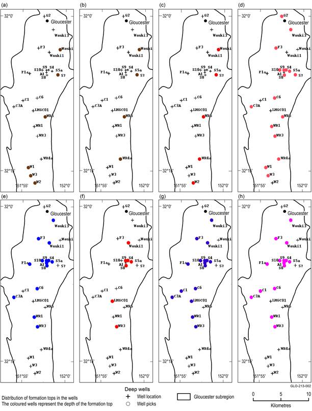
The coloured wells are those that contain a formation top: (a) Alum Mountain Volcanics, (b) Durallie Road Formation, (c) Mammy Johnsons Formation, (d) Waukivory Creek Formation, (e) Dog Trap Creek Formation, (f) Speldon Formation, (g) Wenham Formation and (h) Jilleon Formation.

The different formations are figured in different colours.

‘Well picks’ are the markers of the formation top depths in the wells.

See Table 3 for well acronyms and Table 4 for more details about the well picks.

The 1 second STRM data from the DEM (see Section 2.1.2.1.2) were extrapolated with a local B‑spline algorithm to produce a topographic surface for the geological modelling domain (Figure 8). The local B-spline algorithm calculates the amplitude of a family of bell-shaped functions (B-splines) using a local heuristic approach. The sum of these functions defines a function in (x, y) that approaches the input data.

Figure 8 Surface topography map above the coal-bearing geological Gloucester Basin area modelled in three dimensions

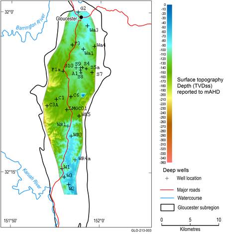
TVDss = total vertical depth subsea reported to the Australian Height Datum; negative values represent elevation above sea level

See Table 3 for well acronyms.

Data: NSW Trade and Investment (Dataset 1); Bioregional Assessment Programme (Dataset 2); Geoscience Australia (Dataset 4)

2.1.2.2.3 Three-dimensional non-faulted and non-eroded geological model

The three-dimensional non-faulted and non-eroded geological model building is an intermediary step in the modelling process. Intermediary non-faulted and non-eroded isopach maps are built on the base of the well data extrapolation and then intermediary non-faulted and non-eroded depth maps are computed on the base of a reference horizon, that is, the top of the Wenham Formation. This process is explained in the modelling workflow, Section 2.1.2.2.1. The intermediary maps of thickness (isopach maps) and depth are not to be taken as real geological results. They just represent a step in the modelling and the trends observed, and do not necessarily correspond to current geological formation depth or thickness variations.

The top of the Wenham Formation was selected as the reference horizon as it represents the shallowest formation top with the highest number of well picks (16 wells) (Figure 7 ).

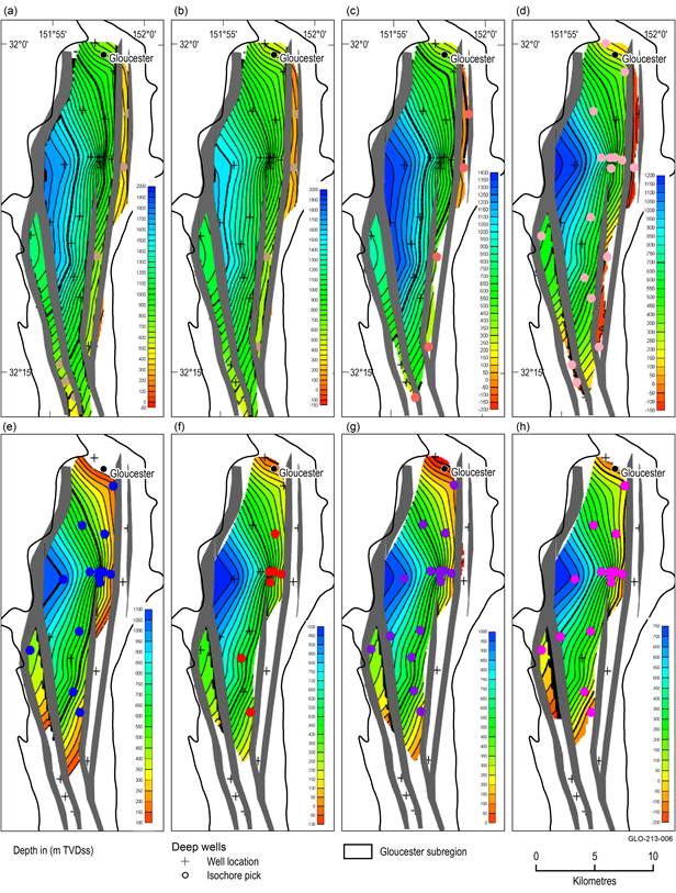
Isopach data were determined directly from the twenty-four selected wells. Seven isopach maps were extrapolated (Figure 9):

For isopach maps (a), (b), (c) and (g), general thickness trends were determined from the formation thickness data deduced from the well picks (isochore data) showed on Figure 9. For isopach maps (d), (e) and (f), no trend was adequately defined for the Gloucester subregion and a general thickness was used.

The resulting isopach maps are nondeterministic and the uncertainty increases as the isochore data concentration decreases. Note that these isopachs correspond to an intermediary step in the modelling and do not represent the final isopachs observed in the geological Gloucester basin. For their determinations only the well data and unfaulted models are considered, virtually eroding them toward the edges of the basin by the creation of the ‘faulted final model’.

Figure 9 Isopach maps containing distribution of formation thicknesses in the wells derived dataset (24 wells) for the coal-bearing geological Gloucester Basin area modelled in three dimensions

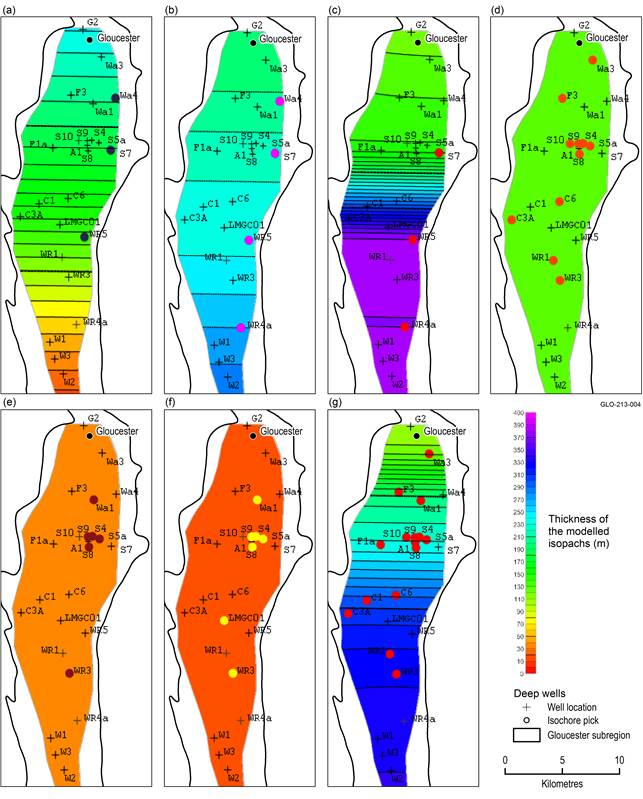
(a) Top Alum Mountain Volcanics to top Durallie Road Formation, (b) Top Durallie Road Formation to top Mammy Johnsons Formation, (c) Top Mammy Johnsons Formation to top Waukivory Creek Formation, (d) Top Waukivory Creek Formation to top Dog Trap Creek Formation, (e) Top Dog Trap Creek Formation to top Speldon Formation, (f) Top Speldon Formation to top Wenham Formation and (g) Top Wenham Formation to top Jilleon Formation.

See Table 3 for well acronyms.

Data: NSW Trade and Investment (Dataset 1)

The horizon depth map (Figure 10) was created using a radial basis algorithm with a 50 m lateral step (x and y). This algorithm provides a good approximation of scattered data by forming linear combinations of radial functions centred at each data point. Please refer to the RMS Roxar website (Emerson, 2016) for more details.

The resulting horizon depth map is nondeterministic with uncertainty increasing as data concentration decreases.

The structural map of the top of the Wenham Formation and the isopach maps (Figure 9) were used to build a non-faulted and non-eroded geological model. This model has a horizontal resolution of 200 by 200 m (x, y), with 50 vertical layers for a total of 501,000 cells. The depth ranges between +818 mAHD and –1830 mAHD.

Figure 10 shows depth structure maps of the non-faulted and non-eroded formation tops extracted from the geological model.

Figure 10 Depth structure maps of non-faulted and non-eroded horizons extracted from the coal-bearing geological Gloucester Basin area modelled in three dimensions

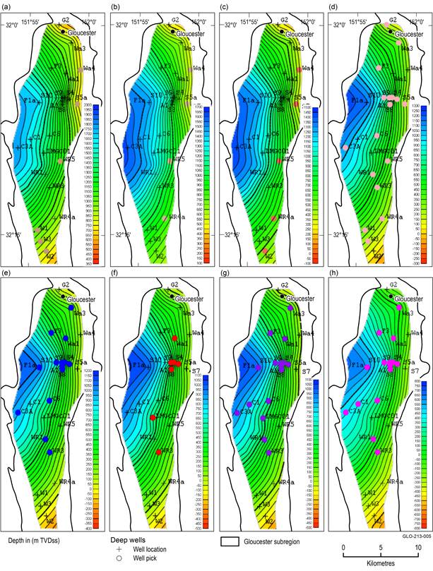
(a) Alum Mountain Volcanics, (b) Durallie Road Formation, (c) Mammy Johnsons Formation, (d) Waukivory Creek Formation, (e) Dog Trap Creek Formation, (f) Speldon Formation, (g) Wenham Formation and (h) Jilleon Formation.

‘Well picks’ are the markers of the formation top depths in the wells.

TVDss = total vertical depth subsea reported to the Australian Height Datum; negative values represent elevation above sea level; different colour scales are used for each map

See Table 3 for well acronyms.

Data: NSW Trade and Investment (Dataset 1)

2.1.2.2.4 Fault analysis

Major fault trends and displacements were incorporated in the model to obtain a faulted geological model. These fault trends were estimated from the observation of the geological map (location of the edges of the basin) and included to accommodate visible misfits (greater than 100 m) between the extracted non-faulted and non-eroded horizons (Figure 10) and the formation tops at wells (Figure 7).

This model was then eroded using the present-day surface topography. The final eroded and faulted model (Figure 11) has a horizontal resolution of 200 by 200 m (x, y), with 50 vertical layers for a total of 501,000 cells. The depth ranges between +665 mAHD and –1755 mAHD.

Figure 11 Three-dimensional perspective view of the eroded and faulted geological model for the Gloucester subregion - diagram in the top left-hand corner shows vertical sections within the model

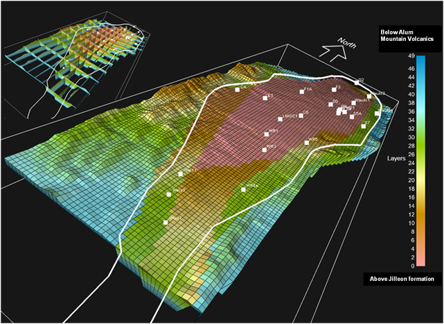
Figure 12 shows the formation tops extracted from the eroded and faulted geological model. The main fault trends affect the stratigraphic pile and are localised along the western and eastern flanks of the Gloucester subregion. The trends located within the subregion accommodate a normal displacement which varies between 200 and 500 m. The other fault trends, which fit the geological limit of the subregion, accommodate normal displacements up to 1000 m.

Figure 12 Depth structure maps extracted from the eroded and faulted geological model for the coal-bearing geological Gloucester Basin area modelled in three dimensions

(a) Alum Mountain Volcanics, (b) Durallie Road Formation, (c) Mammy Johnsons Formation, (d) Waukivory Creek Formation, (e) Dog Trap Creek Formation, (f) Speldon Formation, (g) Wenham Formation Wards River Conglomerate and (h) Jilleon Formation

TVDss = total vertical depth subsea reported to the Australian Height Datum; negative values represent elevation above sea level – grey lines represent the main fault trends

Data: NSW Trade and Investment (Dataset 1); Bioregional Assessment Programme (Dataset 2); Geoscience Australia (Dataset 4)

A fault size population is defined by plotting the fault size (here maximum displacement) versus the cumulative number of faults (e.g. Yielding et al., 1996). An observed characteristic of many sampled fault populations is that the size-frequency distribution is described by a power-law of the form:

where N is the number of features having a displacement greater than or equal to D, a is a measure of the size of the sample and C is the power-law exponent. On a plot of log N against log D, a power-law distribution is defined by a straight line segment with slope –C. The population distribution can be used to extrapolate fault size outside the sampling range and predict sub-seismic scale faults and to validate structural interpretations.

A fault size population for the Stratford CSG Prospect area was defined according to the structural interpretation of Grieves and Saunders (2003). This population can be used to constrain and calibrate the large faults in the geological model and also to predict smaller faults that have the potential to affect connectivity of coal seams and aquitards.

For instance, eighteen normal faults with measurable throw are mapped on the Top Bowen Rd split 5 (BR5 – see companion product 1.1 for the Gloucester subregion (McVicar et al., 2014) for details) horizon for the approximately 7 km² Stratford CSG Prospect area (Grieves and Saunders, 2003) (Figure 13a). The reported throws range from 100 to 10 m. Using a typical power-law slope of –1 (e.g. Yielding et al., 1996; Needham and Yielding, 1996; Bailey et al., 2005; Manzocchi et al., 2009), two fault populations (Stratford medium case and Stratford lower case) are proposed for the Stratford CSG Prospect area (Figure 13b and Figure 13c). Comparison with other fault populations that had been estimated in the coal-bearing Permian basins, that is Collie Basin (WA) (Figure 13d) and the Taranaki Basin (New Zealand) (Figure 13e), scaled down to the same surface area (approximately 7 km²), suggests that the Stratford CSG Prospect area fault population (Figure 13a) could be (i) overestimated (e.g. due to over interpretation of the seismic data) and/or (ii) the displacement for these faults are overestimated (e.g. due to inaccurate horizon picking or time depth conversion). Figure 13f shows the fault size population extrapolated from the Stratford lower case fault population upscaled to the size of the Gloucester geological basin (220 km²). It shows a higher cumulative number of faults than other fault populations from the coal-bearing Permian Collie Basin in WA (Figure 13g) and the East Pennine Coalfield in UK (EPC) (Figure 13h). This again suggests a possible overestimation of the fault size and displacement in the Stratford and Gloucester populations. A fault population for the Gloucester subregion similar to the Collie Basin (Figure 13g) would yield larger faults with maximum displacement around 1500 m which correlate with the faults needed to accommodate displacement in the geological model.

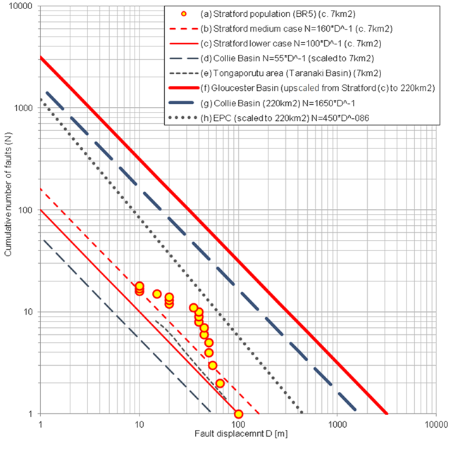
Figure 13 Fault size populations for the Gloucester subregion

Dots represent the Gloucester Gas Project fault data derived from Grieves and Saunders (2003). Thin lines (b, c, d and e) represent population scaled to the size of the Gloucester Gas Project (c. 7km²). Thick lines (f, g and h) represent population scaled to the size of the Gloucester subregion; log scale is used