The major assumptions and model choices underpinning the Galilee subregion GW AEM are listed in Table 15. The goal of the table is to provide a non-technical audience with a systematic overview of the model assumptions, their justification and effect on predictions, as judged by the modelling team. This table is aimed to assist in an open and transparent review of the modelling.
In the table, each assumption is scored on four attributes using three levels: high, medium and low. Beneath the table, each of the assumptions is discussed in detail, including the rationale for the scoring. The ‘data’ attribute is the degree to which the question ‘if more or different data were available, would this assumption/choice still have been made?’ would be answered positively. A ‘low’ score means that the assumption is not influenced by data availability while a ‘high’ score would indicate that this choice would be revisited if more data were available. Closely related is the ‘resources’ attribute. This column captures the extent to which resources available for the analysis and processing of the available data and the modelling, such as computing resources, personnel and time, influenced this assumption or model choice. This attribute explicitly does not consider spending additional resources on data acquisition, as this is covered in the data attribute. Again, a ‘low’ score indicates the same assumption would have been made with unlimited resources, while a ‘high’ value indicates the assumption is driven by resource constraints. The ‘technical’ attribute deals with the technical and computational issues. A score of ‘high’ is assigned to assumptions and model choices that are dominantly driven by computational or technical limitations of the model code. These include issues related to spatial and temporal resolution of the models.
The final and most important column, ‘effect on predictions’, addresses the ‘so what?’ question, the effect of the assumption or model choice on the predictions. This is a qualitative assessment by the modelling team of the extent to which a model choice will affect the model predictions, with ‘low’ indicating a minimal effect and ‘high’ a large effect. Especially for the assumptions with a large potential impact on the predictions, it will be discussed that the precautionary principle is applied; that is, the hydrological change is over estimated rather than under estimated.
While this table is primarily intended to elaborate on the effects of model assumptions and choices, it can provide guidance for further research. A large number of assumptions in the Galilee subregion are mainly driven by the limited data and knowledge base. The effect on predictions column indicates which ones are considered to have the largest effect on predictions. The conclusions and opportunities section (Section 2.6.2.9) uses this table to identify the main data and knowledge gaps.
Table 15 Qualitative uncertainty analysis as used for the Galilee subregion
2.6.2.8.2.1 Layer cake geology – mean layer thickness
The analytic element modelling framework implemented in TTim (Bakker, 2015) only allows representing a groundwater system as a layer cake (i.e. all hydrostratigraphic units are horizontal and have a uniform thickness).
This assumption is therefore driven by technical constraints, not the availability of data or resources, as a three-dimensional geological model of the Galilee subregion has been developed by the Assessment team (see Section 2.1.2 in companion product 2.1-2.2 for the Galilee subregion (Evans et al., 2018a)). The data and resources columns are scored ‘low’ accordingly, while the technical attribute is scored ‘high’.
The effect on the predictions of drawdown of not fully accounting for the geometry of the hydrostratigraphic units is considered small, at least in the confined part of the groundwater system. In a confined system, aquifer geometry only affects groundwater flow through its effect on the transmissivity. Evaluating a wide range of hydraulic conductivity values in the uncertainty analysis de facto means that a wide range of transmissivity values are evaluated. Conceptually, the uncertainty in aquifer geometry is absorbed in the variability of hydraulic conductivity. This is illustrated in the comparison of the analytic element model results and the MODFLOW model results, which shows that the drawdown predictions are comparable, despite the differences in simulated geometry in both models.
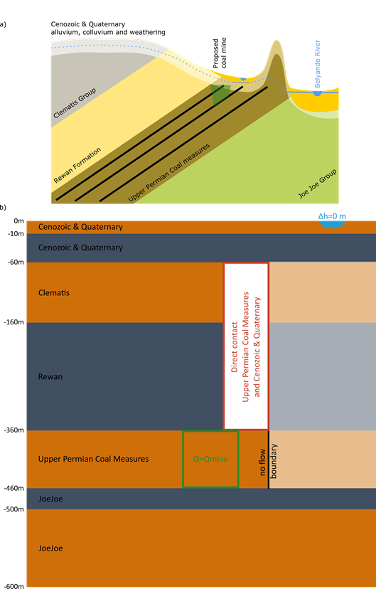
The local absence of model layers, such as the eastern limit of the extent of the Clematis Group and upper Permian coal measures, is accounted for by allowing direct contact between upper Permian coal measures and the alluvium where Clematis Group is absent and by a no-flow boundary at the eastern limit of the upper Permian coal measures.
In unconfined groundwater flow systems, especially in systems like the alluvium and Cenozoic aquifer with a highly variable geometry and a thin saturated zone, groundwater flow is more likely to be controlled by variations in geometry. The representation of the Cenozoic hydrostratigraphic unit is discussed in greater detail in Section 2.6.2.8.2.6.
The overall effect on predictions is scored ‘medium’, which reflects that the layer cake assumption will mostly have an effect on the predictions in the Cenozoic and alluvial sediments and will have much less effect on the confined aquifers.
2.6.2.8.2.2 Principle of superposition – direct simulation of change
A crucial assumption in the analytic element model is the validity of the principle of superposition; that is, that solutions to the groundwater flow equations are additive as long as the system behaves linearly, as outlined in Section 2.6.2.1. This assumption allows for simulating the change in the system due to coal resource development directly, rather than to simulate all fluxes and stores for two different futures and obtain the change as the difference between those two futures. This assumption allows the exclusion of processes that are not affected by coal resource development, such as regional diffuse recharge, from the modelling.
The data analysis in companion product 2.1-2.2 for the Galilee subregion (Evans et al., 2018a) highlighted the limited data availability on the current groundwater flow conditions in the Galilee sedimentary basin. The data attribute is nevertheless scored ‘medium’. The reasoning behind this scoring is that additional data would only warrant to revisit the assumption if the principle of superposition would be shown not to be applicable; that is, if the additional data show that the aquifers in the Galilee Basin do not behave as a confined groundwater system.
The resources and technical attributes are both scored ‘low’ to reflect that this model choice is not driven by operational constraints or technical limitations.
The effect on predictions is scored ‘low’ as Reilly et al. (1987) and Rassam et al. (2004) showed that for mild violations of the linearity assumptions, the deviations in predictions caused by the non-linearity are generally very small and only become apparent in extreme cases. As processes such as regional diffuse recharge are not simulated and therefore cannot compensate for the coal mining related drawdown, the simulated drawdown can be considered as conservative.
2.6.2.8.2.3 Spatially uniform hydraulic properties
The transmissivity (the product of hydraulic conductivity and layer thickness) and storage are considered spatially uniform, at least in the horizontal direction.
The limited data available on these hydraulic properties does show that these properties are heterogeneous (companion product 2.1-2.2 for the Galilee subregion (Evans et al., 2018a)). Furthermore, changes to hydraulic properties due to longwall mining activities are not accounted for in this model. The data density is, however, too limited to empirically establish a spatial correlation structure to characterise the spatial variability in these properties. The sparse head observation dataset does not allow for estimating spatial variability through inverse modelling. The data attribute is therefore scored ‘high’.
Incorporating spatial variability in the modelling would require additional resources as it takes time to develop spatial fields from the available data. In addition to that, incorporating spatial variability will increase the dimensionality of the parameter space. This increases the computational load as more model runs need to be added to the design of experiment to fully explore the larger parameter space. As the analytic element model has very short runtimes, the resources attribute is scored ‘low’.
The analytic element code is not designed to handle spatial variability in hydraulic properties. The technical column is therefore scored ‘high’.
The effect on prediction is scored ‘low’. Groundwater level and flux estimates, especially at the regional scale, are dominated by the bulk hydraulic properties (Barnett et al., 2012). Companion submethodology M07 (as listed in Table 1) for groundwater modelling (Crosbie et al., 2016) illustrates that the probabilistic approach adopted in the bioregional assessments ensures that by varying the uniform hydraulic conductivity stochastically, the effects of spatial heterogeneity are captured in the predictive distributions of change in groundwater level. At a local scale, however, within a kilometre of a stress such as an open-cut mine, spatial heterogeneity is important (Crosbie et al., 2016).
2.6.2.8.2.4 Upper Permian coal measures as single layer
The upper Permian coal measures is not a single aquifer, but a heterogeneous alternation of coal seams and interburden layers. While at least locally the stratigraphic information is sufficiently detailed to split this hydrostratigraphic unit into separate units, the Assessment team decided against doing so, mainly because of difficulties with implementing the CRDP. The CRDP is implemented by assigning the individual proponent’s mine dewatering rates from the relevant environmental impact statements (EISs) to the mine footprint. Insufficient information is available at present to distribute this pumping rate to separate units within the upper Permian coal measures for all proposed mines in the region. The data attribute is therefore scored ‘medium’, while the resources and technical attributes are scored ‘low’.
Moore et al. (2015) illustrated that the way coal seams are amalgamated in groundwater models in the context of dual-phase flow when simulating effects of coal seam gas extraction can have an impact on predictions. Figure 25 therefore explores the effect of lumping all pumping together into a single layer on drawdowns. A seven-layer confined aquifer system is simulated with an analytic element model, in which three coal seams (CS) with a thickness of 4 m each are interspersed in between interburden layers (IB) with a thickness of 22 m each. Each coal seam is dewatered to its base elevation for a period of 30 years. The total resulting pumping rate is assigned to a single layer with hydraulic conductivity and storage equivalent to the seven-layer aquifer. The horizontal hydraulic conductivity of the coal seams is set to 0.1 m/d and the interburden to 0.001 m/d. The vertical hydraulic conductivity is ten times lower than horizontal hydraulic conductivity. The storage coefficient for coal seams and interburden are the same and equal to 1x10⁻⁶ 1/m. Initial conditions are set to zero metres for all layers.
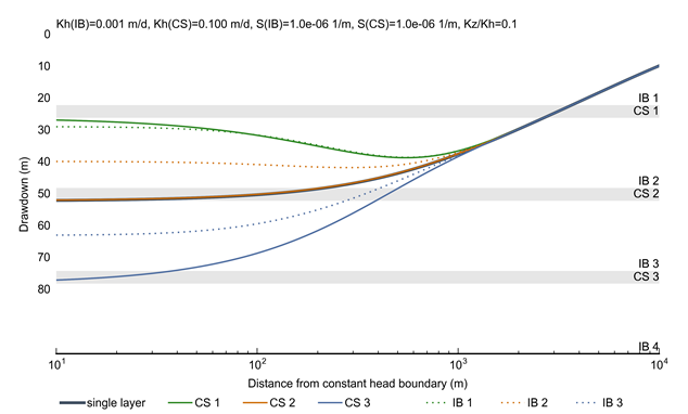
A seven-layer confined aquifer system is simulated with an analytic element model, in which three coal seams (CS) with a thickness of 4 m each are interspersed in between interburden layers (IB) with a thickness of 22 m each. Each CS is dewatered to its base elevation. The total resulting pumping rate is assigned to a single layer with hydraulic conductivity and storage equivalent to the seven-layer aquifer.
Figure 25 shows that the drawdown in the individual coal seams increases with depth. The equivalent drawdown in the single layer corresponds to the drawdown in coal seam 2. At the base of the overlying aquitard, the Rewan Group, the single-layer approach chosen for the regional-scale analytic element model over estimates drawdown, compared to the drawdown simulated at the base of the aquitard in the multi-layer model (IB 1). The overall effect on predictions is therefore scored ‘medium’.
2.6.2.8.2.5 Belyando River alluvium as zero groundwater level change boundary condition
The only surface water – groundwater interaction represented in the GW AEM is the main channel of the Belyando River. The Belyando River is considered a regional groundwater discharge feature that controls the groundwater levels either through baseflow contribution to the Belyando River or through evapotranspiration of the riparian vegetation. As this is not affected by coal mining, the change in groundwater level underneath the Belyando River is set at a constant level equal to zero metres. In effect, this is the same as the implementation of the river boundary condition in MODFLOW, where the river stage is specified independently from any mine development.
From the potentiometric surface of the Cenozoic aquifer in companion product 2.1-2.2 for the Galilee subregion (Evans et al., 2018a) it can be inferred that the Belyando River is the only surface water feature that is not considered to be maximally losing; that is, where groundwater levels are sufficiently far below the river bed elevation for the magnitude of the surface water – groundwater flux to become independent from the hydraulic gradient (Brunner et al., 2009). This potentiometric map is, however, based on very few groundwater-level and river-stage observations. It is very likely that this assumption will need to be revisited when more data are available to inform the river connection status. The data attribute is therefore scored ‘high’.
The resources and technical attributes are both scored ‘low’ to reflect that the choice for this boundary condition is not influenced by operational or technical constraints.
This boundary condition obviously affects the drawdown predictions in the immediate vicinity of the Belyando River and therefore it can potentially lead to an underestimate of the drawdown if it should transpire that the Belyando River is maximally losing. Other streams, however, such as Native Companion Creek and Carmichael River, are not represented in the model. This implies that in the vicinity of those streams drawdown will be over estimated if these streams are not maximally losing.
Implementing the zero groundwater level change boundary results in an estimate of the change in surface water – groundwater flux. In this implementation it accounts for both changes in baseflow to the Belyando River and changes in the local evapotranspiration by riparian vegetation. The change in flux is integrated in the surface water modelling as a change in groundwater flow contribution to streamflow. As the change in evapotranspiration flux is included in this estimate, the change in baseflow flux will always be over estimated and the assumption can be considered to be conservative in the Belyando River channel.
For the other streams in the modelled region, baseflow contribution will not change if the maximally losing assumption is valid. The GW AEM will therefore potentially under estimate the change in baseflow, should this be proven not the case.
For Carmichael River it is noteworthy that part of the baseflow is provided by Doongmabulla Springs, which are sourced from the Clematis Group. The median of the additional drawdown at this location in the Clematis Group aquifer is about 2 m. The resulting change in spring flow is not simulated as no information is available on the hydraulic conductivity of these springs and the fraction of spring flow that contributes to Carmichael River.
The effect on predictions is scored ‘high’.
2.6.2.8.2.6 Representation of the Cenozoic and alluvial aquifer systems
The Cenozoic and alluvial aquifer systems are represented as a layer of infinite extent, with a constant bottom elevation and a saturated thickness of at least 10 m.
From Section 2.1.2.2.5 in companion product 2.1-2.2 for the Galilee subregion (Evans et al., 2018a) it is clear that the presence, extent, nature and thickness of Cenozoic and alluvial sediments is very variable. Drillhole data commonly lack detail in the description of these sediments. While a potentiometric surface for the Cenozoic is presented in Section 2.1.3.3.2 (Figure 53), the combined uncertainty in this surface and bottom elevation surface make it difficult to create a reliable map of the saturated thickness. The data availability is therefore scored ‘high’ for this assumption.
The technical attribute is scored ‘medium’ as it is possible with analytic element code to represent areas where the cover sediments are not present. Varying the thickness or bottom elevation, however, is not possible. Note that representing such thin, discontinuous aquifers will generally give rise to strong hydraulic gradients which are challenging to solve with the current generation of finite difference, element and volume solvers for groundwater flow equations.
The resources attribute is scored ‘medium’, mostly to reflect that the local information on the cover sediments held by mining companies is not yet incorporated in the geological model.
Representing the Cenozoic cover sediments as infinite in extent leads to an overprediction of the extent of drawdown, but can locally lead to an underprediction of the drawdown. The overall effect is therefore scored ‘high’.
2.6.2.8.2.7 Implementation of the coal resource development pathway
The mines are implemented as time series of specified pumping rates assigned to the mine footprints. In the Cenozoic and alluvial aquifers, a constant change in groundwater level of 10 m is assigned to reflect the complete removal and dewatering of the overburden.
To estimate the water production rates of the mines in the groundwater model, detailed information is needed on the geometry of the coal seams, the local hydrogeological properties and the mine progression plans. The pumping rates estimated in the EIS reports by the individual mines are currently considered the best integration of local information.
While the open-cut mines will remove overburden and therefore dewater the Cenozoic and alluvial aquifers, it is not clear from the available data (see previous discussion in Section 2.6.2.8.2.6) that these sediments are present at the mine location and have a saturated thickness of 10 m.
The data attribute is therefore scored ‘high’. The resources attribute is scored ‘low’ to reflect that this model choice is not dominated by operational constraints. The technical attribute is scored ‘low’ as it is possible to implement mines differently, such as through time-varying drainage levels in TTim.
The effect on predictions is scored ‘high’. In the confined parts of the system, the predicted drawdown is linearly related to the pumping rate; that is, a doubling of the pumping rate will result in a doubling of the drawdown (Reilly et al., 1987).
This relationship does not hold in the unconfined part as the specified boundary conditions represent a complete dewatering of the aquifer. The saturated thickness decreases close to the mine which means that the transmissivity of the aquifer, the product of hydraulic conductivity and saturated thickness, is no longer constant. Figure 26 explores the effect of this assumption by comparing drawdown in an unconfined aquifer cross-sectional model estimated with the analytic element code, assuming constant hydraulic properties, and a MODFLOW-2005 model (Harbaugh, 2005), in which transmissivity and storage vary spatially depending on the saturated thickness. An unconfined aquifer is considered with a horizontal hydraulic conductivity of 5 m/d and specific yield of 0.1. The base and top of the aquifer are both uniform and respectively set at –10 m and zero metres. Initial groundwater levels are set equal to the aquifer top at zero metres. A cross-sectional model is created, where the x-dimension is 10,000 m and the y-dimension 100 m. The y‑direction is discretised in only one grid cell (one row of cells). The x-direction has a 100 m grid resolution (100 columns of cells). This grid resolution is representative of the discretisation that in practice can be achieved in regional-scale groundwater models. A constant head boundary of –10 m is introduced at x=zero metres representing constant drawdown due to mine dewatering. To mimic the infinite aquifer extent of the analytic element model in MODFLOW, a constant head boundary equal to zero metres is set at x=10,000 m. The intercell transmissivity is computed by the arithmetic mean of saturated thickness and logarithmic mean of hydraulic conductivity, as advised in Harbaugh (2005) for unconfined aquifers with gradually varying transmissivity.
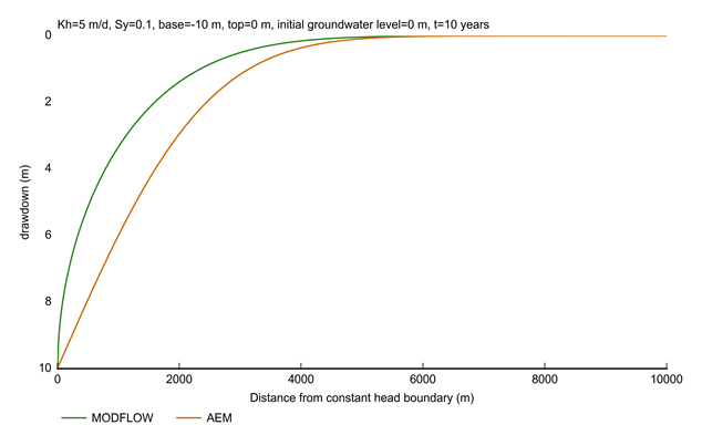
Aquifer is unconfined, with a constant thickness of 10 m. The cross-sectional model is 100 m wide and 10,000 m long. At x=10,000 m a drawdown of zero metres is specified in the MODFLOW models. No lateral boundaries are specified for the analytic element model.
Figure 26 shows that the drawdown by the analytic element model is larger than the drawdown simulated with the MODFLOW model. Dewatering the aquifer reduces the transmissivity to almost zero in the close vicinity of the constant head boundary. Low transmissivities allow for steeper gradients, hence the smaller drawdowns in the MODFLOW model. Transmissivity is constant in the analytic element model which means the gradient will be less steep and therefore estimated drawdown will be larger. This analysis shows the use of the analytic element model is conservative for drawdown predictions in the unconfined aquifer.
Applying a specified drawdown of 10 m in the unconfined aquifer, however, does require the unconfined aquifer to be present and to have a saturated thickness of at least 10 m. As pointed out in Section 2.6.2.8.2.6, this assumption is not justified everywhere, especially further away from the mine areas (further discussion of the spatial extent and thickness of the Quaternary alluvium and Cenozoic sediment aquifer in the area of the modelled coal mines is provided in companion product 3-4 (Lewis et al., 2018) for the Galilee subregion). This means that there is a propensity for the predictions to be overly conservative. To explore this, an alternative conceptualisation is evaluated in which the constant drawdown boundary condition is removed (Figure 27).
The same set of 10,000 posterior parameter combinations as presented in Section 2.6.2.8.1 are evaluated with this alternative conceptualisation.
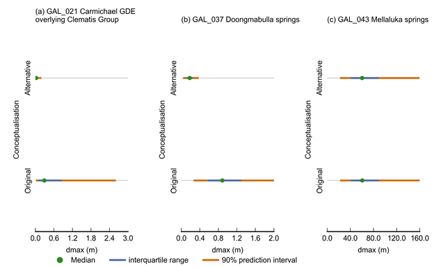
Additional drawdown is dmax, the maximum difference in drawdown between the coal resource development pathway (CRDP) and baseline, due to additional coal resource development.
GDE = groundwater-dependent ecosystem
Figure 28 shows the boxplots of maximum drawdown for both conceptualisations for the model nodes associated with the Carmichael groundwater-dependent ecosystem (GDE) overlying Clematis Group (GAL_021, unconfined Cenozoic and Quaternary), Doongmabulla Springs (GAL_037, confined Clematis) and Mellaluka Springs (GAL_043, confined upper Permian). The plot shows that the removal of this constant drawdown boundary condition has a very large effect on model nodes GAL_021 and GAL_037. The median dmax values at Carmichael GDE decrease from 0.29 m to 0.02 m, while at Doongmabulla Springs, the median dmax values drop from 0.88 m to 0.18 m. The dmax values at Mellaluka Springs are not noticeably affected by the conceptual change.
These results highlight that locally, in the vicinity of the mines, in the unconfined Cenozoic sediment and Quaternary alluvial aquifer and the underlying confined Clematis aquifer, most of the simulated drawdown is caused by the constant drawdown boundary in the unconfined aquifer, which assumes a continuous unconfined aquifer with a saturated thickness of 10 m. When this assumption is not valid, the predictions can be over estimated by up to an order of magnitude.
Despite its closer proximity to the mine, the dmax values at the Carmichael GDE are smaller than these at Doongmabulla Springs. This is because the model node associated with Doongmabulla Springs is situated in the confined Clematis aquifer (see Section 3.5 of companion product 3-4 (Lewis et al., 2018) for the Galilee subregion for further discussion of the likely source aquifer for the Doongmabulla Springs complex), where the storage is orders of magnitude smaller than in the overlying unconfined aquifer in which the Carmichael GDE model nodes are situated. For the same change in flux, the smaller storage will lead to larger drawdown.
The two conceptualisations evaluated using the analytic element model for the Galilee subregion (as described above) are the focus of more detailed discussion presented in Section 3.3.2 of companion product 3-4 (Lewis et al., 2018). In particular, the analysis in Lewis et al. (2018) explores how the different conceptual frameworks affect the application of the regional-scale groundwater modelling results, especially for the local (i.e. point-scale) assessment of potential drawdown impacts at some locations in the vicinity of the seven proposed coal mines modelled for this BA (such as Doongmabulla Springs).
2.6.2.8.2.8 Unconstrained posterior parameter distributions
The posterior parameter distributions are estimated by the Assessment team, informed by the locally available measurements. The relatively large ranges specified for these parameters reflect the confidence the Assessment team has in the estimates. The GW AEM is designed to simulate change directly, not to reproduce historical conditions. It is therefore not possible to infer or constrain model parameters by fitting the model to historical observations of groundwater level or flux.
The data attribute is scored ‘high’ as there are very limited measured data available on the hydraulic properties of the system. Resources are scored ‘medium’ as operational constraints did not allow for the establishment of a formal expert elicitation of model parameter prior distributions. The technical attribute is scored ‘low’ as it is straightforward to change the parameter distributions.
The effect on predictions is scored ‘medium’. A change in posterior parameter distributions will result in different predictions. The wide range of these parameters, however, makes the predictions conservative.
Although constraining the parameters with historical state observations is not possible with the current implementation of the GW AEM, it is unlikely that the current historical observations have sufficient information to greatly constrain the parameters relevant to the predictions. Figure 3-14 in Turvey et al. (2015), for instance, shows that the calibration metric is not very sensitive to some of the most important parameters for drawdown prediction, such as the hydraulic properties of the upper Permian coal measures. A similar conclusion was reached in companion product 2.6.2 (groundwater modelling) for the Clarence-Moreton bioregion (Cui et al., 2016), where the historical observations were shown to be unable to constrain the parameters relevant to the predictions.
2.6.2.8.2.9 Maximum drawdown not realised during simulation period
Across the Bioregional Assessment Programme, the simulation period is chosen to be from 2012 to 2102 as discussed in companion submethodology M06 (as listed in Table 1) for surface water modelling (Viney, 2016) and companion submethodology M07 (as listed in Table 1) for groundwater modelling (Crosbie et al., 2016). For some parameter combinations and some model nodes this means that the additional drawdown is not realised within the simulation period.
Extending the simulation period is not limited by data as it is about the future, hence the score ‘low’. The resources attribute is, however, scored ‘high’. Ensuring that the drawdown is realised at all model nodes for all parameter combinations would require extending the simulation period with hundreds to even thousands of years. This would impose a sizeable increase in the computational demand and therefore compromise the comprehensive probabilistic assessment of predictions. The technical attribute is scored ‘low’ as it is trivial to extend the simulation period.
The effect on predictions, however, is scored ‘low’. The theoretical assessment of the relationship between dmax and tmax presented in companion submethodology M07 (as listed in Table 1) for groundwater modelling (Crosbie et al., 2016) shows that the drawdown decreases with increasing year of maximum change. It can be shown that any additional drawdown realised after 2102 will always be smaller than the drawdowns realised before 2102. This is in line with the precautionary principle as it means that by limiting the simulation period, the hydrological change will not be under estimated.
In the Cenozoic and Clematis Group aquifers, the drawdown is dominated by the specified drawdown in the Cenozoic aquifer, which is 10 m. This drawdown is specified for the entire simulation period to represent that a non-rehabilitated open pit will continue to drain a shallow unconfined aquifer, even after mining operations cease. As this stress operates for the entire simulation period, it is unlikely that the maximum drawdown is realised within the simulation period in the Cenozoic and Clematis Group aquifers. This drawdown will, however, by design, not exceed 10 m. In order to simulate the year of maximum change, mine rehabilitation plans need to be incorporated to represent when the aquifer is restored to pre-mining conditions. These site-specific details are beyond scope and highly speculative.
2.6.2.8.2.10 Model nodes assigned to hydrostratigraphic units
This is scored ‘medium’ in the data attribute as, with the exception of some springs, it is generally well known which hydrostratigraphic unit a model node sources water from. Resources are also scored ‘medium’. The technical attribute is scored ‘medium’ as the vertical resolution of the model is not sufficient to assign some model nodes to the correct hydrostratigraphic unit. An example is model node GAL_039, Spring 107A, which has the Ronlow beds as water source but is assigned to the underlying Clematis Group layer.
Any misclassification has the potential to greatly affect the predictions as the difference in drawdown can be an order of magnitude for different hydrostratigraphic units at the same location. The effect on predictions is therefore scored ‘medium’.
