2.1.4.2 Statistical analysis and interpolation

2.1.4.2.1 River cross-sections at simulation nodes

In Australia, cross-section data are generally available at streamflow gauges only. River model simulations are required to assess the impacts of coal resource development on streamflow at several locations where cross-section data are lacking. Obtaining channel cross-sections requires detailed surveys which are time-consuming and carried out under stringent guidelines (Stewardson et al., 2005). Regional hydraulic geometry models can be obtained using proxies (catchment area, mean annual streamflow) that are more readily available. Using data from about 400 stations in Queensland, Tennakoon and Marsh (2007) developed functional relationships of modest explanatory value (with a coefficient of determination r²≈0.3) between cross-section width and mean channel depth with catchment area and mean annual streamflow. A similar approach was used here to produce stream cross-sections in headwater catchments where there is no upstream gauge (so that the averaging method described in Section 2.1.4.1.2 is not applicable), by assuming that cross-sections at nearby gauging stations (or at gauging stations draining a comparable catchment area, or at gauging stations with comparable mean annual streamflow) provided a reasonable estimate of bottom channel width (Bioregional Assessment Programme, Dataset 3). The information on bottom channel width (L) was then converted into a Cippoletti weir (Figure 34) with a height (H) able to accommodate AWRA-L maximum streamflow.

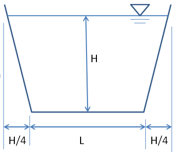
Figure 34 Cross-section of a Cippoletti (trapezoidal) weir

H=height, L=bottom channel width

The flow equation for a trapezoidal Cippoletti weir with side slopes vertical to horizontal ratio of 4 to 1 estimates height (H) for a given flow Q as:

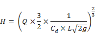
where C_d is the coefficient of discharge (assumed as 0.62; Daugherty and Franzini, 1965), g is gravity acceleration (9.81 ms^-2). C_d considers roughness of the channel (e.g. Manning’s n) and other variables that govern flow and channel cross-sectional area relationship and it can be adjusted to match maximum flow height for a nearby catchment. This process may be simplistic and there are no suitable data to evaluate the approach. Methods exist that use DEMs to estimate cross-sections (Patro et al., 2009), but they require high resolution data currently not available for the geographic domain (see Teng et al., 2015). The Cippoletti weir cross-sections do not incorporate overbank geometry, which means that this assumption may be reasonable in the headwater catchments for which the cross-sections have been derived, as they tend to drain rapidly (due to the steeper down-valley gradients) only after intense rainfall events, which will very unlikely overtop the stream bank. Again systematic errors arising may be partially compensated through calibration. Furthermore, as the Bioregional Assessment Programme is reporting on the relative difference of hydrological response variables between baseline and the coal resource development pathway (CRDP), any errors introduced by the above assumptions will partially cancel out. Table 10 shows the characteristics of the 22 derived cross-sections.

Table 10 Characteristics and dimensions (used in the Cippoletti weir) of derived cross-sections used in AWRA-R modelling for the Hunter subregion

AWRA-R = Australian Water Resources Assessment river model

Data: Bioregional Assessments Programme (Dataset 3)

For seven nodes that were between or close to existing gauges, the cross-section of the closer gauge or gauge with similar catchment area was chosen to define its cross-section. Table 11 shows the characteristics and cross-section used in these locations. These were added to the calibration node-link network, defining the simulation node-link network (CSIRO, Dataset 5). Again, distances between gauges vary from a few to tens of kilometres, which may result in over- or underestimation of the river channel geometry when choosing the upstream or downstream cross-sections. Model calibration will partially compensate proportional biases arising from this underestimation.

Table 11 Characteristics of derived cross-sections used in AWRA-R modelling for the Hunter subregion

AWRA-R = Australian Water Resources Assessment river model

Data: Bioregional Assessments Programme (Dataset 3)

2.1.4.2.2 River reach lengths

River reach lengths are used in AWRA-R to compute instream actual evapotranspiration and rainfall fluxes, instream capacity and groundwater recharge from an irrigated area (Lerat et al., 2013; Dutta et al., 2014).

River reach lengths are quantified for all rivers in the reach, including main channel and tributary channels (if these exist) (CSIRO, Dataset 4). River reach lengths are obtained from the River Styles spatial layer for NSW, which was obtained through digitisation of high resolution aerial or satellite imagery with field validation from many different sources (NSW Department of Primary Industries (Office of Water), Dataset 6). Visual assessment showed that these data were more accurate than drainage networks derived from DEM data, particularly in meandering sections of the river. The dataset was clipped using catchment boundaries defined by the AWRA-R modelling domain (see Section 2.6.1.3 in companion product 2.6.1 for the Hunter subregion (Zhang et al., 2018); CSIRO Land and Water, Dataset 7) and each river reach length was manually selected using GIS software and lengths computed. These lengths are planar and are different from real lengths, particularly in steep areas.

2.1.4.2.3 Irrigation areas and crop types

The AWRA-R river model needs details of irrigated areas and crop types in each river reach in which irrigation is present in order to determine areal extent and crop factors of the most common crop types (Dutta et al., 2015).

Areas and crop types are obtained from the Catchment scale Land Use Management (CLUM) (described in Section 2.1.1; Department of Agriculture: Australian Bureau of Agricultural and Resource Economics and Sciences, Dataset 8). The dataset was clipped using catchment boundaries defined by the AWRA-R modelling domain (see Section 2.6.1.3 in companion product 2.6.1 for the Hunter subregion (Zhang et al., 2018); CSIRO Land and Water, Dataset 7) and the information summarised by reach in order to determine crop types and associated crop factors (CSIRO Land and Water, Dataset 9). Irrigation areas are determined using the first level classification in the CLUM dataset which describes the main land use type. Crop types were determined from the third level classification, which provides detailed information on crop types. A summary of areas and crop types per river reach is shown in Table 12.

Table 12 Crop types and areas used for modelling in each AWRA-R reach for the Hunter subregion

AWRA-R = Australian Water Resources Assessment river model

Data: CSIRO Land and Water (Dataset 9)

2.1.4.2.4 Hunter River Salinity Trading Scheme discharges

The purpose of the Hunter River Salinity Trading Scheme (HRSTS) is to manage river salinity to ensure suitable outcomes for agriculture, mining, electricity generation, town water supply and other uses by using a system of salt credits (NSW Environment Protection Authority, 2003). Mines discharge saline water collected in mine pits and shafts to continue with their operations, and electricity generators discharge water used for cooling that is more saline due to evaporation leading to more concentration of natural salt. The scheme has been devised so that participants in the scheme (mines and electricity generators) can only discharge saline water when conditions in the receiving stream are such that the mixing is below a certain threshold (measured in electrical conductivity units or EC). Three sectors in the river are considered: upper, middle and lower, delimited by three gauging stations (Table 14). In addition, in each sector three streamflow thresholds determine how scheme participants can release saline water. During low-flow conditions, no discharges are allowed. During high-flow conditions, limited discharge is allowed and controlled by the salt credit system in which members of the scheme coordinate discharges to abide by the HRSTS. During flood conditions, unlimited discharges are allowed as long as the salt concentration does not go above 900 EC (NSW Environment Protection Authority, 2003).

Discharge data (NSW Environment Protection Authority, Dataset 10) from scheme participants were analysed to determine timing and discharge volumes under the different flow conditions (Bioregional Assessment Programme, Dataset 1) for the above mentioned sectors. The NSW Environment Protection Authority (EPA) dataset provided observed discharge volumes and EC data for eleven sites, including two sites in the upper sector (mining), four sites for the middle sector (three mining and one electricity generation), and five sites for the lower sector (four mining and one electricity generation), which have gauging stations nearby with observed daily streamflow data. The water discharge records for the three sectors were for the years 2006 to 2012. The lower sector had 217 discharge records from 2007 to 2012, whereas the middle sector had 345 records for the period from 2006 to 2012. The upper sector only had 12 discharge records for the years 2008 to 2012. Details for each site considered in the analysis are presented in Table 13.

Table 13 Details for sites in the Hunter River Salinity Trading Scheme (HRSTS) with discharge records

Data: NSW Environment Protection Authority (Dataset 10)

Water quality is not considered in the surface water modelling for the bioregional assessment of the Hunter subregion, however discharge from participants in the scheme may impact water quantity and thus hydrological response variables. Thus, simple rules for mine and electricity generation water discharge were devised and implemented in AWRA-R. The following assumptions were made in the estimation:

Although there were only up to six years of discharge data, a pattern between discharge and rainfall was examined. As pointed out previously, it was hypothesised that mines and electricity generators would need to do more dewatering in a wetter climate and there would also be more opportunities for discharging. Conversely, less dewatering would be needed in a drier climate alongside less opportunities for discharge. Therefore, wet and dry years were identified by using the mean annual long-term rainfall from 1973 to 2014. Years above average (wet) were 2007, 2008, 2010 and 2011, whereas 2009 and 2012 were below average (dry) years. Figure 35 shows discharge volumes for all individual discharges in each HRSTS sector were grouped into wet and dry years and combined to produce a daily discharge. Note that under these criteria there were only three discharge events in the upper sector during dry years. Although water discharge is somewhat lower during dry years, the differences are not important when compared to high-flow conditions. Consequently, discharge volumes (see below) in the model were not varied to reflect wet and dry years.

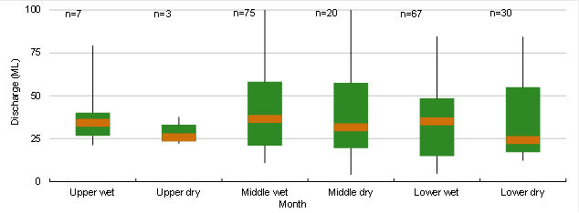
Figure 35 Box plots of water discharge for each sector during dry and wet years

Orange identifies the median value; green boxes define the interquartile ranges; whiskers indicate the 10th and 90th percentiles of discharges. Individual scheme participant discharges are combined in each sector for dry and wet years to produce a daily discharge.

HRSTS = Hunter River Salinity Trading Scheme; n is the number of discharge events in each sector for dry and wet years

Data: NSW Environment Protection Authority (Dataset 10)

The NSW EPA data were used to estimate annual releases to obtain a mean annual release by river sector. Also individual releases were used to estimate a ratio of discharge to streamflow volume (Table 14). In the model, it is assumed that scheme participants can discharge water up to a volume determined by the mean annual release. The amount discharged once the streamflow threshold is exceeded is determined by the fixed ratio of water, which depends on the streamflow volume. Discharge is computed daily, which is the temporal resolution of observed streamflow data and modelling time-step (see Section 2.6.1.3 in companion product 2.6.1 for the Hunter subregion (Zhang et al., 2018)). In dry years when the streamflow threshold may not be exceeded very often, scheme participants may not be able to discharge all their mean annual volume. It is assumed that the water that cannot be discharged is reused or otherwise disposed of. In wet years, when there are more opportunities for discharge, scheme participants will often discharge the full mean annual water discharge volume.

Table 14 Gauges, streamflow thresholds and mean annual discharge volumes and discharge/streamflow ratio used in the simplified discharge scheme for the Hunter subregion

Data: Bioregional Assessment Programme (Dataset 1), NSW Environment Protection Authority (Dataset 10)

2.1.4.2.5 Node-link interpolation

The AWRA-R model generates outputs at model nodes. In order to characterise the changes in stream hydrology from additional coal resource development throughout the Hunter River modelling domain, results from the model nodes must be interpolated or extrapolated to reaches (links) in the river network for which results are not specifically computed. Companion submethodology M06 (as listed in Table 1) for surface water modelling (Viney, 2016) details the approach. In general, results at a model node are assumed to apply to some length of reach upstream and downstream of the node, so far as there is no significant change in the hydrology along the reach. Where a change in flow could occur, such as from a tributary inflow or hydrological changes caused by mining, it is not appropriate to interpolate from the model nodes beyond this point of difference.

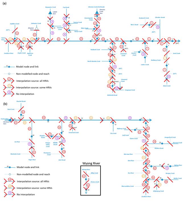
The interpolation (link to node mapping) is informed by analysis of Google Earth imagery and GIS layers of mine footprints, stream network and subcatchment areas. Figure 36 shows the link to node mapping for the modelled link-node networks of the Hunter River and Wyong River (not to scale): red lines delineate distinct reaches, each of which is associated with a number in a circle, corresponding to a model node, or to a cross in a circle, indicating that an interpolation cannot be made. Non-model reaches (dashed blue lines) have been added to identify inflows to model links where results from a model node are no longer applicable; and non-model nodes (open blue circles) have been included to identify points along a reach where some other change in hydrology, such as a coal mine or tidal influence, renders the interpolation inaccurate. Table 15 lists the non-model nodes and provides details of their location.

Figure 36 Link-node mapping for (a) the lower Hunter River and (b) upper Hunter, Goulburn and Wyong River modelled river networks

HRV = hydrological response variable

Not all tributary inflows are deemed to cause a noticeable hydrological change to the receiving stream. Small inflows into much larger streams, such as from Unnamed Creek at node 11 into the Hunter River, do not affect the interpolation along the receiving reach – that is, results from node 10 are assumed applicable both upstream and downstream of the inflow point; whereas larger inflows can cause a sufficiently large hydrological change such that results from an upstream node can be applied only to the reach upstream of the junction and results from the downstream node applied only to the reach downstream of the junction. This is illustrated where Wollombi Brook joins the Hunter River, with the Hunter River reach upstream of the junction mapped to node 20 and the reach downstream of the junction mapped to node 10.

Table 15 Location details of non-model nodes used to inform the Hunter River link-node mapping

At the most downstream point of the link-node network, results from node 1 (stream gauge 210064 on Hunter River at Greta) can be extrapolated to the tidal limit of the Hunter River. This is represented in Figure 36 (a) by non-model node (X9*) and corresponds to the point on the Hunter River where the rail line crosses the river.

Extrapolation upstream of a headwater model node is considered appropriate where there is no coal resource development in the headwater catchment and only as far as the first substantial tributary inflow. An example of this is upstream of node 39 on Baerami Creek. Where there is a coal resource development, such as Ulan mine which is upstream of node 50 on the Goulburn River, no extrapolation is possible.

The interpolation and extrapolation of model results from nodes to stream reaches is used to inform where the receptor impact models (see companion product 2.7 for the Hunter subregion (as listed in Table 2)) can be applied to enable an analysis of risk and impact upon the subregion’s landscape classes and assets (see companion product 3-4 for the Hunter subregion (as listed in Table 2)).