Observed datasets (Section 2.1.2.1) were analysed and processed to form derived datasets for use in the bioregional assessment of the Hunter subregion. These datasets were analysed and interpolated to develop a three-dimensional geological model of the Carboniferous to Triassic stratigraphic sequences of the Hunter subregion. The three-dimensional geological model with 2 km2 cell size was built using Roxar Reservoir Management Software (Roxar RMS). Developed by Emerson (2016), this product is traditionally used in the oil and gas industry to make hydrocarbon reservoir or basin-scale models. Other packages are available, such as GOCAD® Mining Suite or Leapfrog® three-dimensional geological mining software. Roxar RMS was adopted because it has the option of computing 3D facies grids based on a stratigraphic analysis approach within the grid cells (see Emerson (2016) for more details).
2.1.2.2.1 Workflow
Having established the need to build a regional geological model for bioregional assessment purposes, a workflow was defined to construct the first-order subsurface structural and stratigraphic architecture of the Hunter subregion. The approach is based on classical three-dimensional geological modelling approaches (Ross et al., 2004) to produce a simple regional model from poorly constrained datasets. The aim of this workflow is to model the large-scale stratigraphic units without introducing structural complexity into the grid geometry that is not supported by the available hard data (Wellmann et al., 2010). The workflow comprised:
- selection and processing of the observed data to form derived datasets and implementing the model numerical database (see Section 2.1.2.2.2), including:
- defining regional horizons
- determining horizon tops and lithological datasets from the deep well dataset and geological maps
- mapping the topography and bathymetry of the subregion from DEM data
- three-dimensional non-faulted and non-eroded geological modelling (see Section 2.1.2.2.3):
- selecting reference horizons and creating a horizon depth map
- isopach mapping
- building a preliminary (non-faulted and non-eroded) geological model
- extracting depth structure maps from the geological model
- fold and fault analysis to refine the geological model (see Section 2.1.2.2.4).
2.1.2.2.2 Data selection and processing
Spatial distribution of the deep wells data in the Hunter subregion is poor: only heterogeneous scattered well data are available as shown by Figure 6. These types of data are point source and do not provide much insight into the three-dimensional structure of the geological units at depth.
Generalised stratigraphic columns for the Hunter, Newcastle, Western and Central coalfields (shown in the geology section of the companion product 1.1 for the Hunter subregion (McVicar et al., 2015)) and correlations proposed by NSW Trade and Investment (Oliveira et al., 2014) were used to define ‘regional horizons’ for the purpose of this Assessment. Nine regional horizons were determined. They are named according to the nomenclature used by NSW Trade and Investment, with ‘M’ referring to Mesozoic and ‘P’ to Paleozoic. The relationship between these regional horizons and the stratigraphic units in each of the four coalfields are shown in Table 4.
Well completion reports (WCR) were analysed to determine the top depth of regional horizons. Of the 105 wells in the original dataset, 44 wells had information that could be used in the model. The markers of the horizon top depths in the wells are called ‘well picks’. Table 5 summarises for each well in the derived dataset the pick depths and the top of regional horizon to which it corresponds. The uncertainties in the depths to the tops of the horizons are not known. They are a function of the original well stratigraphic interpretation; a new integrated interpretation of all the well logs could remove some uncertainty at this stage. However, due to operational constraints, this type of integrated interpretation could not be achieved for this geological model.
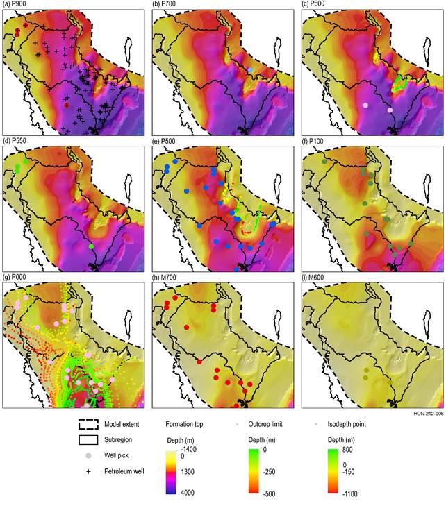
The well top data and relevant structural contours from the outcrop limits and mapped isopachs in the Newcastle Coalfield (see Figure 35 in companion product 1.1) and Western Coalfield (see Figure 36 in companion product 1.1) were mapped for each of the regional horizons (Figure 7). P500 and P100 are the best constrained horizons in terms of number of well tops. Figure 7 shows the distribution of the nine horizon tops in nine separate maps.
Table 4 Relationship between regional horizons and stratigraphic units in the coalfields of the Hunter subregion
Refer to the Sydney Basin stratigraphic column in Hodgkinson et al. (2016) for more details
Table 5 Depth to top of regional horizons from deep wells across the Hunter subregion
aTVD ss = total vertical depth subsea reported to the Australian Height Datum
Data: see the listing of well completion reports within the list of references following Section 2.1.2.3
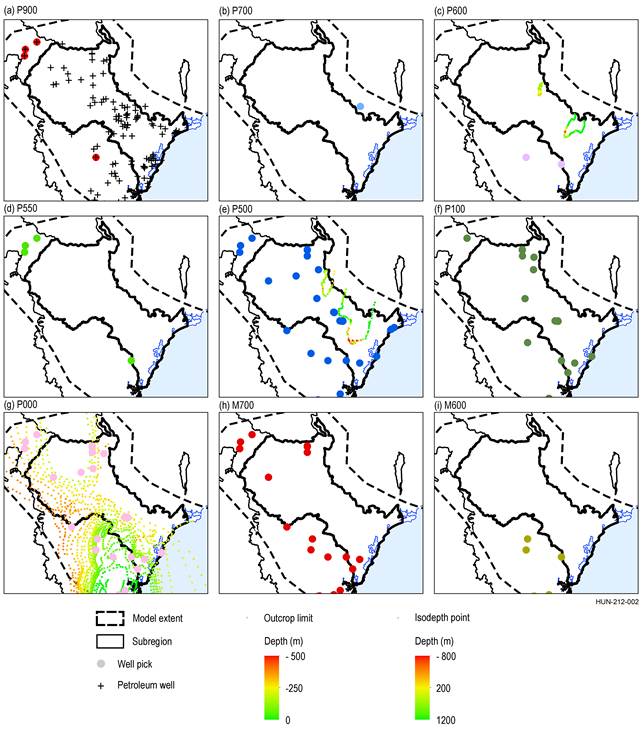
(a) P900 shows all 105 petroleum wells. The 45 well picks that contained sufficient information to define a formation top are coloured differently for each horizon: (a) P900, (b) P700, (c) P600, (d) P550, (e) P500, (f) P100, (g) P000, (h) M700 and (i) M600.
‘Well picks’ are the markers of the formation top depths in the wells.
Outcrop limits are shown for the (c) P600 and (e) P500 horizons.
Isodepth points are shown for (g) P000
Data: DTIRIS NSW (Dataset 1), CSIRO (Dataset 2, Dataset 4), Bioregional Assessment Programme (Dataset 3)
The 3-second DEM and 9-second bathymetry data (see Section 2.1.2.1.1) were extrapolated with a local B-spline algorithm (Roxar package) to produce a topographic and bathymetric map of the Hunter subregion (Figure 8). The local B-spline algorithm calculates the amplitude of a family of bell-shaped functions (B-splines) using a local heuristic approach. The sum of these functions defines a function in (x, y) that approaches the input data: this method generates stable and functional results for all types of mapping (Emerson, 2016).
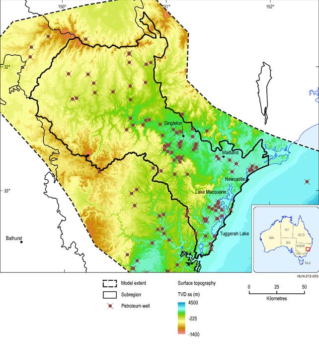
Figure 8 Surface topography and offshore bathymetry of the Hunter subregion
TVD ss = total vertical depth subsea reported to the Australian Height Datum; negative values represent elevation above sea level
Data: Bioregional Assessment Programme (Dataset 3), Geoscience Australia (Dataset 5, Dataset 6)
2.1.2.2.3 Three-dimensional non-faulted and non-eroded geological model
The stratigraphic reference horizons selected for the Sydney Basin geological model of the Hunter subregion were the P900, P500, P100 and P000 horizons (Figure 9). These were chosen because they have the highest density of well picks or are important regional stratigraphic markers in the Sydney Basin (Oliveira et al., 2014).
Horizon P900 is the base of the Sydney Basin sedimentary sequence (i.e. the surface of the geological basement). The horizon depth map for P900 (Figure 9a) was obtained using a global B‑spline algorithm with a 500 m lateral step (x and y). The modelled depth varies between +5780 and –730 m total vertical depth subsea (TVD ss). This reference is used in the well database (Table 5) and is kept in the geological model for consistency purposes. Modelled depths have been compared with the OZ SEEBASE dataset and the calibration with well picks. Basement highs occur onshore along the western and north-east borders of the Sydney Basin; and offshore along a north-east to south-west trend. This basement structure is located deeper than 3000 m below sea level in the central and eastern parts of the basin where thick Permian and Mesozoic sediment layers are observed (purple colours, Figure 9a). This map is an intermediary modelling result that only considers the well picks of P900, without correlation with other structural data and the present-day surface topography.
The P500, P100 and P000 horizons are all important levels within the geological model as they are the stratigraphic boundaries of the main upper Permian coal-bearing units: the Newcastle, Wittingham, Illawarra and Tomago coal measures (Table 4). The initial modelling step maps each horizon independently and does not account for the present-day erosional level (as explained in the workflow, Section 2.1.2.2.1). The horizons were mapped with a 500 m increment in x and y based on the well picks and available mapping data. P500 depth varies between +1830 and –730 m TVD ss, P100 between 1050 and –733 m, P000 between 918 and –796 m. At this stage of the model development, the resulting horizon depth maps are non-deterministic, and the level of geological uncertainty increases proportionally with decreased number of data points. The horizons only conform to the available well data and regional maps, and are not further constrained by other sources of stratigraphic information. This means that there may be a poor level of consistency between different horizons, and in some cases they may even overlap at depth. To build a more coherent stratigraphic model, the next step is to generate isopach maps (thickness maps) of each geological unit, which can be used to constrain the three-dimensional structure of each horizon away from the wells (Figure 9 and Figure 10).
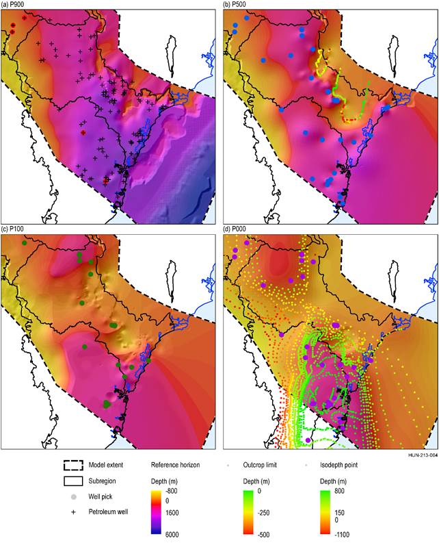
(a) P900 shows all 105 petroleum wells. Well picks used to define formation tops are coloured differently for each horizon.
‘Well picks’ are the markers of the formation top depths in the wells.
Outcrop limits are shown in (b) for the P500 horizon.
Isodepth points are shown for (d) P000
Data: DTIRIS NSW (Dataset 1), CSIRO (Dataset 2, Dataset 4), Bioregional Assessment Programme (Dataset 3)
Six isopach maps were developed by extrapolation away from the calibration points defined by the 44 input wells and with reference to existing mapping (Table 4, Figure 7, Figure 9, Figure 10). The calibration points are called isodepths. An isodepth is the difference between two well picks for a given stratigraphic unit at a given well location. To obtain an isodepth measurement, two consecutive stratigraphic well tops must be available within the well dataset:
- top of P700 to top of P900 – lower Permian volcanic-bearing conglomerate, siltstone and sandstone units of the Dalwood Group
- top of P600 to top of P700 – Greta Coal Measures
- top of P500 to top of P550 – siltstone-dominated units, including Mulbring Siltstone in Newcastle and Hunter coalfields, and Berry Siltstone in Western Coalfield
- top of P000 to top of P100 – upper Permian coal-bearing units including the Newcastle Coal Measures in Hunter and Newcastle coalfields, and Illawarra Coal Measures in the Western Coalfield (base of Narrabeen Group to top of Watts Sandstone)
- top of M700 to top of P000 –Triassic Narrabeen Group
- top of M600 to top of M700 –Hawkesbury Sandstone.
These maps provide a two-dimensional representation of geological unit thickness. For the isopach maps that show the top of P000 to top of P100 (Figure 10d) and top of M700 to top of P000 (Figure 10e), thickness varies between 200 to 790 m and 154 to 789 m, respectively. Thickening occurs from the central Hunter subregion towards the north and south-east of the subregion.
For the other isopach maps, there are no obvious thickness trend variations and a constant thickness has been adopted. Average value of these thicknesses have been determined based on the well pick depths (Table 5) and thickness of formations given in Section 1.1.3.2 of companion product 1.1 (McVicar et al., 2015):
- 365 m for the Dalwood Group (top of P700 to top of P900)
- 88 m for Greta Coal Measures (top of P600 to top of P700)
- 500 m for Mulbring Siltstone in Newcastle and Hunter coalfields and the Berry Siltstone in the Western Coalfield (top of P500 to top of P550)
- 290 m for Hawkesbury Sandstone (top of M600 to top of M700).
The resulting isopach maps are non-deterministic and the uncertainty increases as the isopach data concentration decreases. These isopach maps are another intermediary step in the development of the final geological model and do not represent the final isopach data in the Hunter subregion geological model.
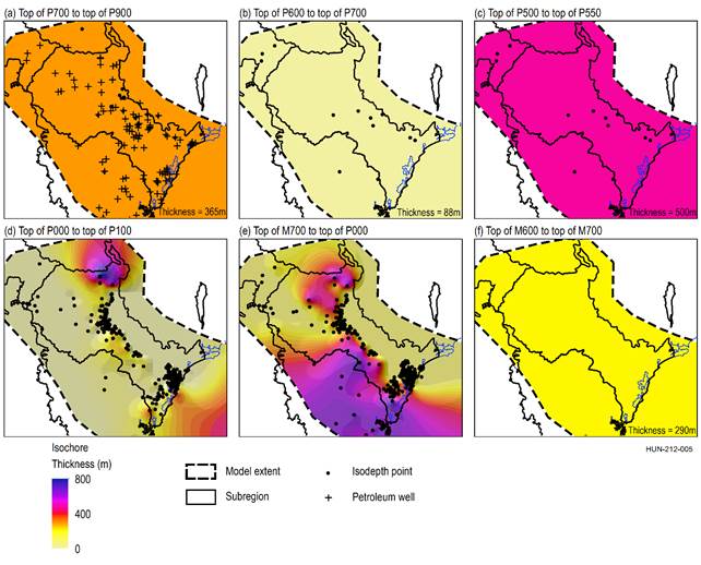
(a) Top of P700 to top of P900, (b) Top of P600 to top of P700, (c) Top of P500 to top of P550, (d) Top of P000 to top of P100, (e) Top of M700 to top of P100 and (f) Top of M600 to top of M700
An isodepth is the difference between two well picks for a given stratigraphic unit at a given well location
Data: DTIRIS NSW (Dataset 1), CSIRO (Dataset 2, Dataset 4), Bioregional Assessment Programme (Dataset 3)
The reference structural maps of P900, P500, P100, P000 (Figure 9) and the isopach maps (Figure 10) were used as input to build a non-faulted and non-eroded geological model. The geological modelling option of the Roxar RMS software takes all this information into account and can generate different simulations depending on the weight given to each dataset. A scenario giving a weight of ‘1’ to the reference horizons and ‘0.5’ to the isopachs was selected. The weighting adjustment is a classical approach in geological modelling, used to minimise the differences between the model results and the input data (Caumon et al., 2009). In this case, the reference horizons are known to be more constrained than the isopachs (Figure 9 and Figure 10) and can thus be used to build the model. The geological modelling option corrects the potential errors in each horizon interpolation, taking into account the interaction between all horizons to respect a minimum thickness between each horizon as well as the geological chronology (for example, P500 cannot occur above P100). This model has a horizontal resolution of 2 km × 2 km (x, y), with 109 layers along the vertical (z) for a total of 511,118 cells. The layers along the vertical can have variable size: 109 layers were adopted to allow a maximum thickness of 200 m to each cell and enable the generation of a facies grid with a non-homogeneous lithology within each unit. The depth ranges between 1185 m above sea level (the highest elevation known in the subregion) and 5062 m below sea level (the deepest part of the sedimentary infill sequence of the Sydney Basin).
Figure 11 shows depth structure maps of the non-faulted and non-eroded horizons extracted from the geological model.
Outcrop limits are shown on (e) and (c) and the isodepth points on (g).
‘Well picks’ are the markers of the formation top depths in the wells.
The depths are in TVD ss AHD = total vertical subsea reported to Australian Height Datum; negative values represent elevation above sea level
Data: DTIRIS NSW (Dataset 1), CSIRO (Dataset 2, Dataset 4), Bioregional Assessment Programme (Dataset 3)
2.1.2.2.4 Preliminary three-dimensional geological model
The extracted non-eroded horizons (Figure 11) were compared with the well data in the geomodelling software (Roxar RMS) and the difference between the datasets was minimised as a function of the main fold trends observed within the Hunter subregion. Then, the resulting horizons were eroded by the topographic level to obtain a preliminary three-dimensional present-day geological model (CSIRO, Dataset 9). Folding seems to be the dominant first-order structure influencing the regional horizon structures: anticline and synclines are indeed the most represented structure within the subregion (Stewart and Alder, 1995).
Fault and fractures are present within the basin but there is insufficient information about their three-dimensional structure, dip, throw and displacement to inform the model in the time frame of the Assessment. Therefore, faults have not been represented in the model (see Section 2.1.2.3).
The three-dimensional structure of the preliminary geological model and the facies distribution within the structural grid are illustrated in Figure 12 and Figure 13. The facies were simply defined at regional scale from the regional generalised stratigraphic column of the Permian and Triassic units in the main coalfields of the Sydney geological basin (Figure 33 of companion product 1.1. for the Hunter subregion (McVicar et al., 2015)). Figure 13 provides an overview of the facies architecture, illustrating the mixed facies of the Permian coal-bearing intervals capped in the central and western parts of the basin by more uniform Triassic sandstone, siltstone and mudstone formations. Figure 14 shows the regional horizon tops extracted from this folded and eroded geological model. The main fold trends affect the entire stratigraphic sequence and the white areas reflect the zones eroded at present day. The model had been folded through several numerical iterations of Roxar RMS stratigraphic modelling plugging to minimise the difference between the primary maps (Figure 11) and the well picks (Table 4). While Figure 14 also shows the surface expressions of faults from previous geological mapping, they are not included in the Hunter geological model.
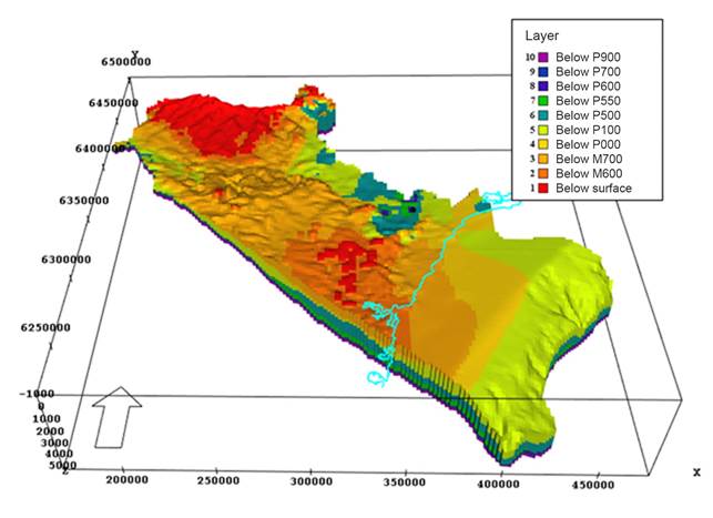
View from the south, showing the surface expression of model horizons across the subregion. Upland areas are dominated by horizon 1; in the more eroded areas, the Newcastle, Tomago, Wittingham and Illawarra Coal Measures (horizons 4 and 5) are at or closer to the surface, and are the main mining areas of the Hunter and Western coalfields where a mix of open-cut and underground mining occur; only underground mining occurs in the Newcastle Coalfield along the coast where the Greta Coal Measures (horizon 8) are deeper.
Data: CSIRO (Dataset 9)
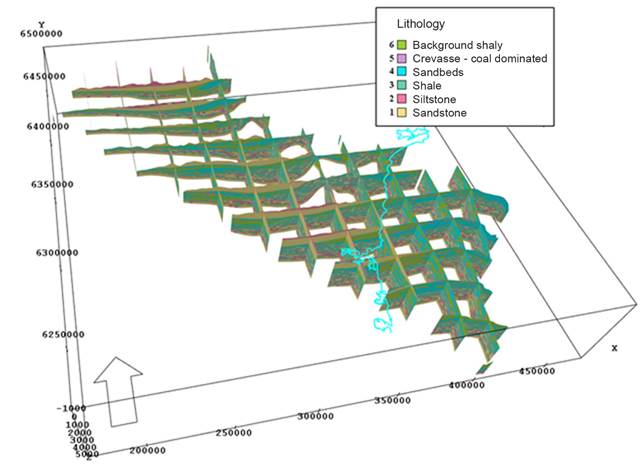
View from the south, showing a change in surface lithology from siltstone and sandstone outcrops in the upland areas of the subregion to shale and sand bed lithologies in more eroded areas. Mining is undertaken in areas where the siltstone and sandstone outcrops have been eroded.
Data: CSIRO (Dataset 9)
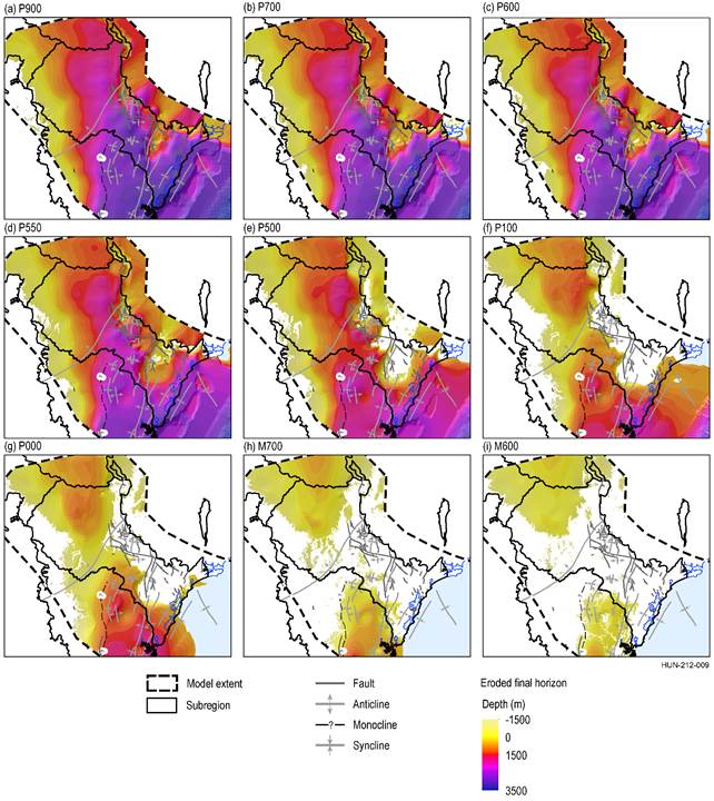
Depth in m TVD ss = total vertical depth to the Australian Height Datum; negative values represent elevation above sea level. Faults from previous geological mapping are shown, but are not included in the Hunter geological model.
Data: CSIRO (Dataset 9)
