2.1.3.2.1 Recharge
Groundwater recharge from rainfall is a crucial input into numerical groundwater models. As there have not been previous estimates of recharge in the Hunter subregion at a scale suitable for the numerical modelling, a gridded recharge surface has been generated for the Hunter subregion using the chloride mass balance method (Anderson, 1945). This simple and cost-effective method for estimating recharge is the most commonly used method in Australia due to the availability of data to support it (Crosbie et al., 2010).
The assumptions that underpin the chloride mass balance method are summarised (Wood, 1999):
- Chloride in groundwater is only sourced from rainfall (not rock weathering or interactions with streams or deeper aquifers).
- Chloride is conservative in the system (no sources or sinks).
- The chloride flux does not change over time (steady-state conditions).
- There is no recycling of chloride in the system (e.g. due to irrigation drainage).
If these assumptions are met, then recharge can be estimated as follows:
|
|
(1) |

where recharge (R) is in mm/year, chloride deposition (D) is in kg/ha/year and the chloride concentration of groundwater [Cl-]gw is in mg/L.
The recharge for the Hunter subregion and Sydney Basin bioregion were estimated together as they are both contained within the geological Sydney Basin. The results for the Sydney Basin bioregion are included here.
The chloride deposition over the geological Sydney Basin was extracted from the national dataset at a resolution of 0.05° (Leaney et al., 2011) (CSIRO, Dataset 13). This dataset was created from 297 field measurements of chloride deposition at point locations and then fitted to the model of Keywood et al. (1997). Figure 20a shows chloride deposition to be much greater near the coast compared to inland areas, which is due to decreasing concentrations of atmospheric salts with distance from the sea.
The chloride concentrations of groundwater were obtained from data collected by NSW Office of Water (now DPI Water) (NSW Office of Water, Dataset 14). There are 1393 points covering several decades of chloride data in the geological Sydney Basin (Figure 20a). A borehole may have one or more observations; where there were multiple observations for a borehole, the geometric mean was used to characterise the chloride concentration, otherwise the isolated value was used. At each location, the chloride data were assigned to a stratigraphic layer based on mapped surface geology (Geoscience Australia, Dataset 15) where better data did not exist. In most cases it was assumed that the bores were completed into the stratigraphic layer representing the surface geology, since there were only a few where the information existed to show otherwise (e.g. bores drilled through Wianamatta Shale to sample the Hawkesbury Sandstone).
In alluvial areas, the chloride signal reflects not only a contribution from rainfall, but also from streams and upward flow from deeper aquifers (Raiber et al., 2016). Consequently, the first assumption of the chloride mass balance method is not met and 529 data points from alluvial areas were excluded from the analysis. The remaining 864 measurements of groundwater chloride concentration were used to calculate point estimates of recharge. Figure 20b shows the spatial distribution of these 864 data points. They are not uniformly distributed across the Sydney Basin with better spatial coverage of recharge estimates in the Hunter subregion.
The second assumption in the chloride mass balance methodology is that the chloride is conservative in the system. In areas without halite deposits it is generally assumed that there are no geological sources of chloride and the trace amounts of vegetation uptake is recycled to the systems as leaves decay.
The assumption of steady-state conditions is difficult to meet in any area where there has been land use change. This can be mitigated by only using shallow bores as the water sampled would be younger. For an area that was cleared 200 years ago with an average recharge rate of 10 mm/year and a porosity of 0.02, the recharge post-clearing would have penetrated 100 m below the water table. If deep bores are used then there is the possibility of having a low bias to the recharge estimates. An attempt was made to only sample younger water by only including bores in the analysis that were screened in the same stratigraphic layer as the surface geology (e.g. bores sampled from the Hawkesbury Sandstone were excluded if they were overlain by the Wianamatta Shale).
The assumption of no recycling of chloride can be achieved by not using bores that are in areas under irrigation.

Figure 20 Inputs into the chloride mass balance method of estimating recharge
Left panel (a) showing the chloride deposition and the chloride concentration of the watertable aquifer and the right panel (b) showing the mean annual rainfall and the point estimates of recharge (excluding points on alluvium)
Data: CSIRO (Dataset 13), NSW Office of Water (Dataset 14), Bureau of Meteorology (Dataset 16), Bioregional Assessment Programme (Dataset 19)
To generate a continuous surface of recharge estimates for input into the groundwater model, the point estimates derived from the chloride mass balance method needed to be upscaled. Crosbie et al. (2010) found that mean annual rainfall, soil type and vegetation type are the key determinants of recharge. Crosbie et al. (2013) used these variables successfully to upscale point estimates to a continuous recharge surface. However, due to the paucity of point recharge estimates under different soil and vegetation types in the geological Sydney Basin, the mean annual rainfall (Bureau of Meteorology, Dataset 16) and eight different classes of surface geology have been used as covariates. The eight geological classes were based on layers defined in the Hunter subregion geological model (see Section 2.1.2.3) with the exception of the near-surface class, which has been split for the purposes of the recharge analysis into three different classes: Dunes (contains coastal dunes, dunes and sandplains), Volcanics (Liverpool Range Volcanics and similar) and Shales (Wianamatta Group and similar).
A log-linear relationship was adopted for estimating mean annual recharge from mean annual rainfall. This is similar to relationships developed previously from both field and modelled data (Crosbie et al., 2013; Crosbie et al., 2010). Use of a log-linear relationship can result in recharge rates at the higher end of the rainfall spectrum that are greater than rainfall (especially when extrapolated beyond the range of the field data). To prevent this, a global maximum recharge rate equal to half the rainfall was imposed, which is approximately the highest recharge estimated from the point scale chloride mass balance estimates. As the chloride mass balance method was not appropriate for alluvial areas, empirical relationships developed from historical field data to predict recharge using mean annual rainfall (Bureau of Meteorology, Dataset 16), soil clay content (Bioregional Assessment Programme, Dataset 17 and vegetation (ABARES, Dataset 18) were used (Wohling et al., 2012).
Figure 21 shows the log-linear relationship for estimating mean annual recharge from mean annual rainfall. This shows that for a given rainfall amount the Dunes, Volcanics and M600 (top of Hawkesbury Sandstone) classes have comparably more recharge than the other classes. The coal-bearing formations (P000) tend to have recharge that is similar to that of the aquitards (Wianamatta Group). Figure 22 shows the upscaled mean annual recharge with the highest recharge along the coast where rainfall is highest on the Dunes, alluvium and M700 (top of the Narrabeen Group); recharge is greatly reduced inland (particularly in the Goulburn river basin). The mean areal recharge across the entire Hunter subregion was estimated to be 23 mm/year. (For the Sydney Basin bioregion, the mean areal recharge was estimated to be 45 mm/year).
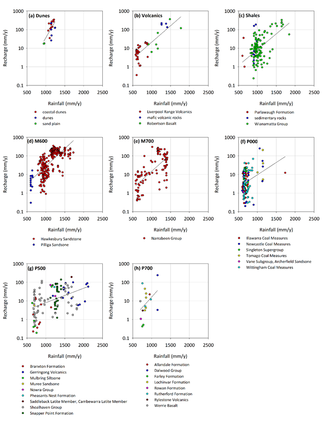
The black line is the line of best fit through the data points. All of the regression lines are significant at a p-value of 0.01 except for P700 (p=0.11).
Data: Bioregional Assessment Programme (Dataset 19)
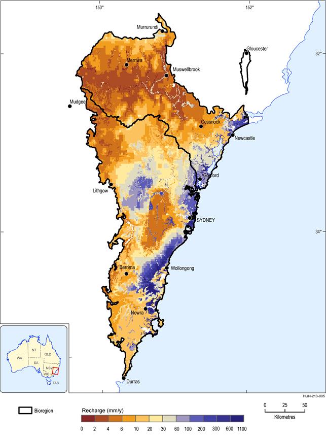
Figure 22 Upscaled estimates of mean annual recharge over the Sydney Basin
Data: Bioregional Assessment Programme (Dataset 4)
The deterministic estimate of recharge shown in Figure 22 was used as the base recharge in the numerical groundwater model. However, an estimate of the uncertainty around this deterministic estimate is necessary for carrying out the sensitivity and uncertainty analyses. The sources of uncertainty that can be quantified are the chloride deposition and the regression function. The chloride deposition shown in Figure 20 is the best estimate reported by Leaney et al. (2011), who also produced gridded estimates of the mean, standard deviation and skewness from 1000 equally well-calibrated replicates (Bioregional Assessment Programme, Dataset 9). These gridded datasets were used to stochastically generate ten alternate chloride deposition grids. Each of these ten deposition grids were used to generate the regression equations between mean annual rainfall and mean annual recharge using bootstrapping (Efron and Tibshirani, 1994) with replacement for ten replicates. This provided 100 replicate regression equations to use in up-scaling (Figure 23). [Bootstrapping is a statistical method that involves random sampling with replacement. In this case it has been used by leaving out some of the data points and replacing them with replicates of other data points and then re-calculating the regression equation. This allows us to estimate the uncertainty in the regression equations developed between rainfall and recharge.]
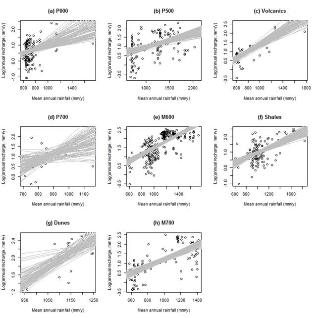
Each line is 1 of 100 replicates of the regression equation between mean annual rainfall and mean annual recharge.
Data: Bureau of Meteorology (Dataset 16), Bioregional Assessment Programme (Dataset 4)
There is a higher uncertainty in the relationships developed for the below P700 class (i.e. below the Greta Coal Measures in the Hunter and Western coalfields) compared to the other classes (Figure 23) due to the lack of data and the spread in the point estimates of recharge. This is reflected in the upscaled estimates of recharge (Figure 24). The areally averaged recharge for the 50th percentile of the 100 replicates is 25 mm/year, with the 5th and 95th percentiles being 21 and 31 mm/year respectively for the Hunter subregion. (For the Sydney Basin bioregion the areally averaged recharge estimates are 35, 42 and 53 mm/year for the 5th, 50th and 95th percentiles respectively.)
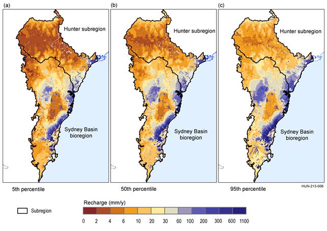
Data: Bioregional Assessment Programme (Dataset 4)
The limitations of the recharge estimation as applied here relate to the assumptions underpinning the methodology: by not accounting for the chloride that is lost from the system through surface runoff, recharge can be overestimated; whereas not accounting for the enhanced deposition on forested areas leads to underestimating recharge. The assumption of steady state conditions will be violated in areas that have not attained equilibrium following the clearing of native vegetation for agriculture, and will likely lead to an underestimation of recharge. No attempt was made to quantify the impacts of such forms of uncertainty.
2.1.3.2.2 Hydraulic conductivity
Hydraulic conductivities control the direction and speed of groundwater flow. Rock layers can be aquitards with low conductivity that retard flow between aquifers, which have higher conductivity. Hence rock conductivity characterises groundwater hydrological connectivity and flow directions.
It is notoriously difficult to appropriately assign a single conductivity to a hydrostratigraphic layer because rocks exhibit strong heterogeneity and anisotropy. Often in groundwater models, a horizontal conductivity and a vertical conductivity are assigned and these are varied by an order of magnitude or more in an uncertainty analysis to simulate the rock’s inherent heterogeneity.
Analyses of hydraulic conductivity measurements from the Hunter subregion were undertaken to determine whether they correlate with the stratigraphic layers of the geological model or the lithologies of the lithological model (Section 2.1.2). The groundwater model is built on these two models, so if any layers or lithologies were found to have a particular hydraulic conductivity, it would inform the parameterisation of the groundwater model. The analysis also informs the uncertainty analysis by placing realistic limits on the variation in hydraulic conductivity.
Hydraulic conductivities and porosities have been measured by mining companies throughout the Hunter subregion for the purpose of characterising their local hydrogeological conditions. The measurements are recorded in environmental impact statements for these mining companies. Five hundred and seventy-seven measurements were selected for analysis because they contained sufficient information to determine their spatial location (including depth), and the hydrostratigraphic unit sampled. They have been compiled into a dataset for the groundwater modelling for the Hunter subregion (Bioregional Assessment Programme, Dataset 9), which includes references to the 21 source documents. The data are highly variable.
Most of the 577 measurements pertain to coal fields and coal-bearing strata, and a significant number are on coal. This introduces some unavoidable bias into the analysis presented below. Measurements are broadly of two types: downhole, where conductivity is measured in the field; and lab, where a rock core is extracted and tested. About 55% of measurements were conducted in the field using various methods, while 20% were performed in the lab. The remaining 25% did not specify the experimental method.
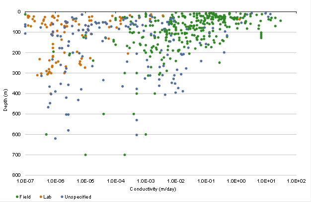
Figure 25 Hydraulic conductivity differentiated by measurement type and correlated with depth
Multiple regression analyses revealed no strong correlation with lithology (Figure 26), Hunter geological model (Section 2.1.2) stratigraphic layers (Figure 27) or geographic area (Figure 28). The measured conductivities for each stratigraphic layer in Figure 27 generally vary by 7 to 8 orders of magnitude, although when the very low conductivities from the lab-based measurements are excluded the range of variability is more like 5 to 6 orders of magnitude. Either way the data show very high intra-layer variability at a regional scale, which means a tightly constrained set of hydraulic conductivity values cannot be specified for each layer.
A similar conclusion is reached when the measurements are classified by lithology (Figure 26). The wide variability in hydraulic conductivity measurements within all lithology classes indicates there is no basis for differentiating between lithologies by hydraulic conductivity at the scale represented by the measurements. A correlation might exist if the hydraulic conductivities for a lithology or stratigraphic layer were biased towards the right (high conductivity) or to the left (low conductivity) in Figure 26 and Figure 27.
The lack of correlation is due in part to the coarse resolution of the regional geological and lithological models, and the challenges presented in attempting to define distinct lithological and stratigraphic characteristics across vast areas from point measurements. The variation in hydraulic properties which might give rise to a particular sequence of aquitards and aquifers at a local scale cannot be assumed to extend over the wider subregion. While there may be distinct geographical differences between sites (e.g. conductivities at one mine site generally being lower than at another mine site, even when the measurements are apparently taken from the same geological layer and lithology), these represent local-scale effects and are largely irrelevant to regional-scale representation of hydrogeology for which variations in hydraulic conductivity over large scales govern groundwater flow. The Hunter groundwater model cannot make direct use of the point-scale hydraulic conductivity data except where it shows a good correlation with regional-scale features, which our analyses indicate it does not. However, such local-scale information can be incorporated into the model emulators. Incorporating local-scale information constrains model predictions in the area where the information is relevant, and this process is demonstrated in companion product 2.6.2 for the Hunter subregion (Herron et al., 2018).
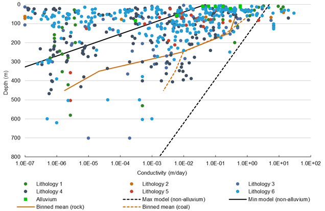
Figure 26 Hydraulic conductivity differentiated by lithology class and correlated with depth
Lithologies are defined in Section 2.1.2 and are: 1, mostly sandstone; 2, mostly siltstone; 3, mostly shale; 4, sandbeds in the fluviatile system; 5, fine sands, silts, and coal; 6, mixture of shale, siltstone and mudstone. The Min and Max model are used by the Hunter groundwater model in the uncertainty analysis (Herron et al., 2018). The Binned mean line shows the arithmetic mean of the conductivity measurements, binned to 100 m depth intervals.
Data: Bioregional Assessment Programme (Dataset 9)
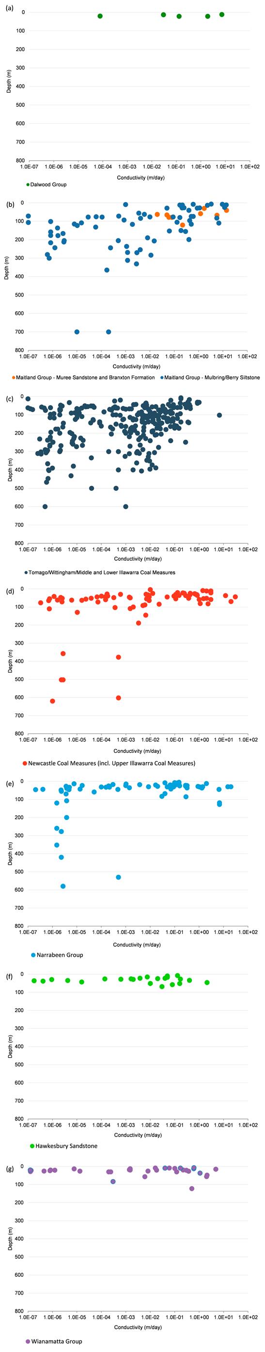
Layer 1 is not shown because there were no data for this layer. While Layer 0 is the lowest stratigraphic layer in the sequence, the measurements correspond to shallow depths, where this layer outcrops at the surface.
Data: Bioregional Assessment Programme (Dataset 9)
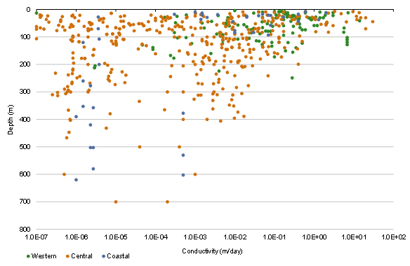
Figure 28 Hydraulic conductivity differentiated by geographic area, and correlated with depth
The various plots show there may be a weak correlation between hydraulic conductivity and depth. In particular, the field-based measurements show a trend of decreasing conductivity with depth (Figure 25), based predominantly on measurements in the Maitland Group stratigraphic units (Figure 27b) and the Tomago, Wittingham and Middle and Lower Illawarra coal measures (Figure 27c). When the data are plotted on a linear scale (Figure 29), it is evident that measurements from the deeper lithologies and stratigraphic layers have hydraulic conductivities less than 0.5 m/day, but there is a lot of variability below this value. The hydraulic conductivity measurements greater than 0.5 m/day are almost all within the top 100 m. As discussed previously, the large degree of scatter is due to the different test types, different formations being sampled and the inherent heterogeneity of rocks and sediments.
While the correlation is weak, Figure 26, Figure 27 and Figure 29 suggest that representing hydraulic conductivity as a function of depth in the Hunter groundwater model is more accurate than adopting a constant hydraulic conductivity throughout. The bold lines (Max model and Min model lines) shown in Figure 26 correspond to the maximum and minimum hydraulic conductivity values used in the groundwater model uncertainty analysis, which are discussed further in companion product 2.6.2 for the Hunter subregion (Herron et al., 2018).
The binned-mean line in Figure 26 shows the arithmetic mean, which is biased to the higher hydraulic conductivity measurements, for each 100 m depth increment. It is used to inform the parameterisation of the Hunter groundwater model, as flow at the large scale is governed by preferential pathways of high conductivity. A small region of low conductivity is almost irrelevant at the large scale. This pattern can be observed in Figure 25, which distinguishes the measurements by testing type. The downhole field tests typically yield higher conductivities than lab methods because: (1) a successful coring requires reasonably coherent rock with few fractures, while downhole measurements may be sampling a highly fractured region (Rovey and Cherkauer, 1995); and (2), the groundwater flows through preferential pathways of high conductivity. The depth-decay functions presented in the figures above (‘Max model’ and ‘Min model’) more accurately capture measurements at larger scales than at the scale of cores. This is discussed further in Herron et al. (2018).
Figure 28 distinguishes the conductivity measurements by geographical area. Most data come from the ‘Central’ area (Hunter Coalfield), so the depth decay function used most accurately captures the hydraulic conductivities in that region. The data are more limited for the other two areas and the quantitative form of the depth decay is less clear, especially in the ‘Western’ area (Western Coalfield) where measurement depths are concentrated within the top 150 m with relatively few measurements at greater depths. Nevertheless, the ‘Max model’ and ‘Min model’ conductivities used in the uncertainty analysis bound the plausible range of conductivities in all regions. Similar depth relationships have been used in the Hunter subregion previously. For example, correlations with depth reported in AGE (2012) and AGE (2014) lie between the maximum and minimum shown in Figure 26, and Figure 13 in companion submethodology M07 (as listed in Table 1) for groundwater modelling (Crosbie et al., 2016). Parsons Brinckerhoff (2015) shows a relationship with depth for hydraulic conductivity data from the Hunter, Gloucester and Sydney regions.
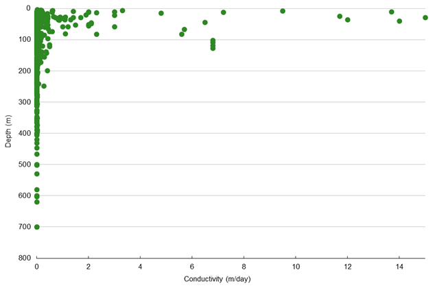
Figure 29 Hydraulic conductivity (on a linear scale) and its relation with depth
Data: Bioregional Assessment Programme (Dataset 9)
When measurements were classified into alluvium, coal-bearing and rock groupings, the units containing coal are found to be typically up to three orders of magnitude more conductive than the rock that does not contain coal (Figure 30). However, as coal seams are not explicitly represented in the Hunter groundwater model, this distinction is not incorporated into the model.
The alluvium plays an important role in surface water – groundwater interactions. Nine of the 577 measurements pertained to alluvium, and these had mean conductivity of 0.25 m/day (Figure 30). This informs the parameterisation of the Hunter groundwater model.
Comparatively few measurements of porosity were available from the environmental impact statements. The porosity data obtained are shown in Figure 31, along with maximum and minimum values used in the Hunter groundwater uncertainty analysis.
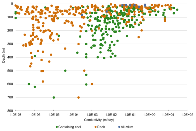
Figure 30 Hydraulic conductivity for coal, rock and alluvium, and correlated with depth
Data: Bioregional Assessment Programme (Dataset 9)
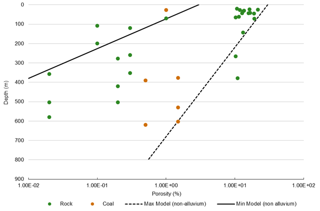
Figure 31 Porosity correlated with depth
Data: Bioregional Assessment Programme (Dataset 9)
