As outlined in the Section 2.6.2.1, the groundwater model is evaluated for a wide range of parameter combinations, called the design of experiment. The results of these model runs, the simulated equivalents to the observations described in Section 2.6.2.7.1 and the predictions described in Section 2.6.2.7.2, are used to train statistical emulators, which will replace the original model in the uncertainty analysis. The range of each parameter sample is therefore chosen to be very wide to ensure sufficient coverage of the parameter space. The design of experiment model runs also allow to carry out a comprehensive sensitivity analysis. Such an analysis provides insight in the functioning of the model, aids in identifying which parameters the predictions are most sensitive to and if the observations are able to constrain these parameters.
Table 8 lists all 62 parameters that have been defined in the groundwater model (see Table 4 in Section 2.6.2.4, Section 2.6.2.5, and Table 6 in Section 2.6.2.6). For each parameter, Table 8 lists the section number where that parameter is defined and described.
To limit and rationalise the dimensionality of the parameter space, not all parameters are included in the sensitivity analysis. The coefficients c and d in the depth – hydraulic conductivity relationship for layers 5 and 6 control the offset and slope of the relationship. While coefficients a and b modify the shape of the relationship, their effect on the resulting hydraulic conductivity is small compared to the slope and offset parameters. Parameters Kx_5_a, Kx_5_b, Kx_6_a and Kx_6_b are therefore excluded from the sensitivity and uncertainty analysis.
The pilot points used to spatially vary the riverbed conductance are included in the analysis. Their values are, however, all tied to parameter rp1. This has the effect that while the value at each of the pilot points changes during the sensitivity analysis, the spatial variability of the riverbed conductance will remain the same. Overall, 38 parameters are changed during the sensitivity and uncertainty analysis.
Table 8 Parameters included in the sensitivity analysis
na = not applicable; Y = yes, included; N = no, not included; parameters are uniformly sampled over their transformed range
Table 8 also lists the transformation of each parameter and their range. Ten-thousand parameter combinations are generated for the entire parameter space for the model sequence (i.e. each parameter combination has parameter values for the groundwater model and the surface water model) using a maximin Latin Hypercube design (see Santner et al., 2003, p. 138). The maximin Latin Hypercube design is generated like a standard Latin Hypercube design, one design point at a time, but with each new point selected to maximise the minimum Euclidean distance between design points in the parameter space. Points in the design span the full range of parameter values in each dimension of the parameter space, but also avoid redundancy among points by maximising the Euclidean distance between two points (since nearby points are likely to have similar model output). The parameter ranges are sampled uniformly from their transformed range (Figure 28).
Within the available time frame and computational resources available, the modelling team was able to evaluate 3,877 out of the 10,000 parameter combinations generated. While the coverage of parameter space is limited with less than 4000 simulations, visual inspection of the successfully evaluated parameters showed that there was adequate coverage of all parameters and no bias or gaps in the sampling of the parameter hyperspace. Section 2.6.2.7.4 describes the development of the emulators with these model results. Part of developing the emulators is verifying that the sampling density is sufficient to train the emulators with an acceptable mismatch between simulated and emulated prediction values.
The following sections describe the sensitivity of the observations and predictions to the 38 parameters. The best appreciation of the relationship between a parameter and an observation or prediction is through the inspection of scatterplots. Although the large dimensionality of parameters, observations and predictions precludes this type of visualisation for all parameter–prediction combinations, a selected few scatterplots are provided as illustration. A comprehensive assessment of sensitivity will be provided through sensitivity indices. These indices, computed using the methodology outlined in Plischke et al. (2013), are a density rather than variance-based quantification of the change in a prediction or observation due to a change in a parameter value. It is a relative metric in which large values indicate high sensitivity, whereas low values indicate low sensitivity.
2.6.2.7.3.1 Simulated equivalents to observations from the design of experiment
Figure 29 shows how the predicted groundwater levels at observation bore CLM_oh6 vary with parameter values. For each parameter the sensitivity index is shown as well. The green line indicates the observed groundwater level. It is very clear that there are a wide range of parameter values that result in predicted groundwater levels matching the observed groundwater level at this location. There are only a few parameters, however, that appear to noticeably affect the predicted groundwater levels:
- DRN_C_2: the drain conductance multiplier for the drain boundary condition at the top of layer 1
- Kx_1_o: the horizontal hydraulic conductivity of layer 1 outside the alluvium
- Kx_4: the horizontal hydraulic conductivity of layer 4
- RCH_2: the recharge multiplier for recharge zone 2.
The other parameters do have an effect on the predicted groundwater levels, but their effect is much smaller than the effect of the four parameters listed above. The sensitivity of the parameters listed is consistent with the understanding of the groundwater system and the design of the numerical model. Increases in recharge (RCH_2) result in higher predicted groundwater levels, while decreases in drainage conductance (DRN_C_2) reduce groundwater outflow out of the model and thus lead to higher groundwater levels. An increase in hydraulic conductivity of layer 1 leads to smaller variations in groundwater level. An increase in hydraulic conductivity of layer 4 allows for a larger fraction of recharge to be transmitted to the deeper basin and therefore lower groundwater levels.
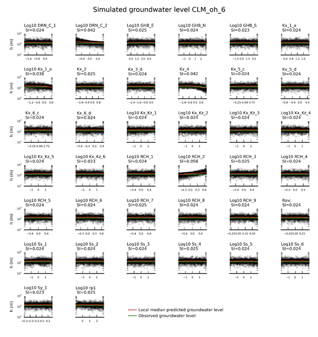
For each parameter, the corresponding sensitivity index (SI) is provided in the title. The sensitivity index is a relative metric in which high values indicate sensitive parameters and low values indicate less sensitive parameters. The red line indicates the local median of simulated values over the parameter ranges spanned by the line segment. The green line is the observed groundwater level.
Figure 30a shows boxplots of the sensitivity indices for all simulated equivalents to the available groundwater level observations. The plot shows that a large number of groundwater level predictions are sensitive to the same set of parameters as identified to be sensitive for groundwater level prediction at observation bore CLM_oh6.
Out of the 38 parameters included in the design of experiment, 9 appear to have a noticeable effect on the simulated groundwater levels. These are:
- GHB_E: the multiplier to the eastern general-head boundary
- RCH_1 and RCH_2: recharge multipliers in zone 1 and 2
- DRN_C_2: the drain conductance multiplier for the drain boundary condition at the top of layer 1
- Kx_1_a, Kx_1_o, Kx_2, Kx_4: the horizontal hydraulic conductivity respectively in the alluvium of layer 1, outside the alluvium in layer 1, layer 2 and in layer 4
- rp1: the conductance of the river boundary condition.
The general-head boundary in the east controls the amount of water entering or leaving the system through the eastern boundary, while parameter rp1 controls the surface water – groundwater flux and thus the amount of water that can leave the system through the river system. As both of these boundary conditions are linear features in the landscape, only simulated groundwater levels close to these boundary conditions are likely to be sensitive to these parameters.
Figure 30b shows the sensitivity to the simulated average surface water – groundwater flux in September and October at the Casino surface water model node location (CLM_008). This prediction is mostly sensitive to the riverbed conductance (rp1), and to a lesser extent to the hydraulic conductivity in layer 1 (Kx_1_a and Kx_1_o) and recharge (RCH_1 and RCH_2).
The final subplot in Figure 30, plot c, shows the sensitivity indices for the total water production rate simulated by the groundwater model. There are 39 sensitivity indices computed, one for each year of CSG water production and one for the total water produced over the entire production period. The simulated CSG water production rates are most sensitive to the drain conductance assigned to the drain boundary condition used to simulate the CSG wells (DRN_C_1) and to the parameters controlling the hydraulic conductivity of the Walloon Coal measures (Kx_6_c and Kx_6_d) and the storage of the Walloon Coal measures (Ss_6).
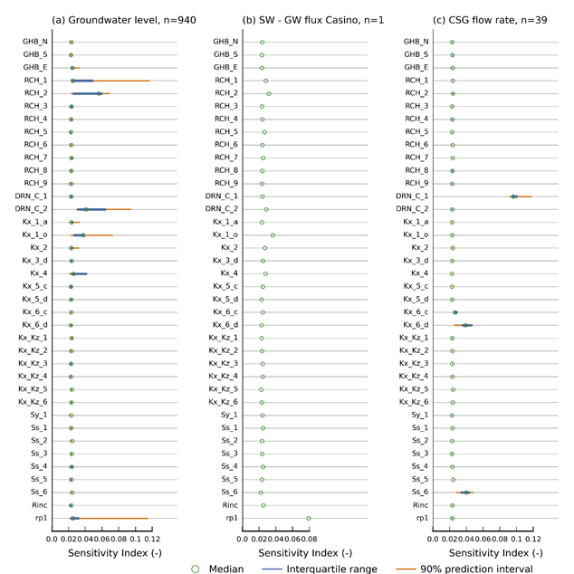
The sensitivity index is a relative metric in which high values indicate sensitive parameters and low values indicate less sensitive parameters
2.6.2.7.3.2 Simulated predictions from the design of experiment
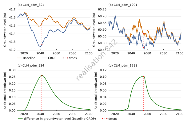
Figure 31 shows, for the results of the evaluated design of experiment runs, how the predicted additional drawdown at model node pdm_1291 varies as a function of the parameter values. Note that additional drawdowns less than the head convergence criterion in the MODFLOW model, which was set to 0.001 m, are truncated to 0.001 m.
The parameters that have a sensitivity index in excess of 0.03 can be considered to have a major effect on the predicted drawdown, in the context of this particular prediction. These parameters are:
- DRN_C_1: the drain conductance assigned to the drain boundary condition used to simulate the CSG wells
- Kx_3_d, Kx_6_d: the horizontal hydraulic conductivity of layers 3 and 6
- Kx_Kz_3, Kx_Kz_5, Kx_Kz_6: the ratio of horizontal to vertical hydraulic conductivity in layers 3, 5 and 6
- Ss_6: the specific storage multiplier for layer 6.
The specific storage multiplier in the Walloon Coal Measures and the drainage conductance multiplier for the CSG drain boundary are the most dominant parameters as they control the water production rate from CSG. The ratios of horizontal to vertical hydraulic conductivity are the next set of important parameters as they control the propagation of the cone of depression through the sedimentary basin. It is noteworthy that increasing the ratio for layers 5 and 6 leads to a decrease in drawdowns, while increasing the ratio for layer 3 leads to increased drawdowns. Increased ratios for layers 5 and 6 implies that the vertical hydraulic conductivity decreases for these layers. Lower vertical hydraulic conductivities impede the propagation of the cone of depression and thus lead to lower additional drawdowns in layer 3. An increase in the ratio of horizontal to vertical hydraulic conductivity in layer 3 also results in lower vertical hydraulic conductivities in layer 3. Lower vertical hydraulic conductivities in layer 3 impede flow from the overlying aquifers into this hydrostratigraphic unit. There will be less compensation of additional drawdown by water from the overlying units and hence higher drawdowns. The horizontal hydraulic conductivities in layers 3 and 6 are important as well as they control the hydraulic conductivity in the source and target hydrostratigraphic units, respectively.
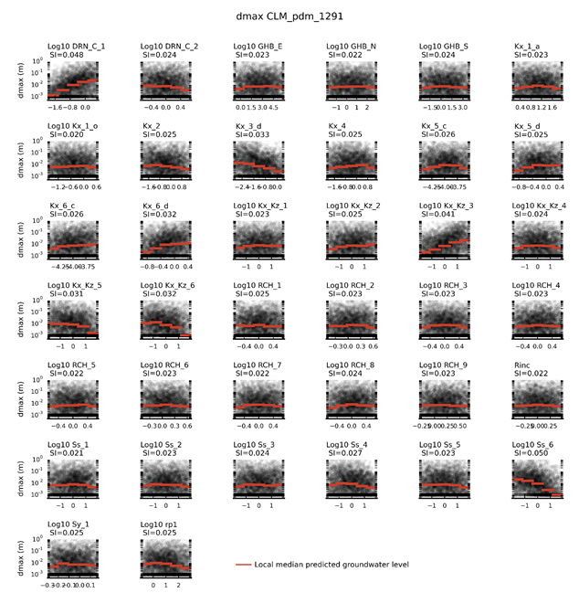
For each parameter, the corresponding sensitivity index (SI) is provided in the title. The sensitivity index is a relative metric in which high values indicate sensitive parameters and low values indicate less sensitive parameters. The red line indicates the local median of simulated values over the parameter ranges spanned by the red line segment.
Additional drawdown is dmax, the maximum difference in drawdown between the coal resource development pathway and baseline, due to additional coal resource development.
Figure 32 shows boxplots of the sensitivity indices for all parameter-prediction combinations. For the additional drawdowns in layers 1, 2, 3, 4 and 6 (Figure 32a to 30e) the same sets of parameters appear to be dominating the predicted drawdown as identified for model node pdm_1291. The most dominant parameter for all layers is the storage multiplier in the Walloon Coal Measures (Ss_6), while the horizontal hydraulic conductivity of the Walloon Coal Measures (Kx_6_d) is less important. The ratio of horizontal to vertical hydraulic conductivity controls the propagation of the cone of depression through the sedimentary sequence and most predictions are sensitive to these parameters. The drain conductance multiplier for the CSG drainage boundary (DRN_C_1) appears most important for predictions in layers 1 to 3 and less so for predictions in layers 4 and 6. This is most likely due to the fact that there are more model nodes close to the CSG well area in layers 1 to 3 than in layers 4 to 6.
The maximum change in historical surface water – groundwater flux (Figure 32f) is most sensitive to the riverbed conductance (rp1). The second-most important parameter is the drainage conductance of the CSG wells, followed by the vertical hydraulic conductivity of layers 5 and 6 and the specific storage multiplier and horizontal hydraulic conductivity for the Walloon Coal Measures (Ss_6 and Kx_6_d). The hydraulic conductivity in layer 4 (Kx_4) appears to be important for the maximum change in surface water – groundwater flux in some reaches.
By comparing Figure 32 and Figure 30 it becomes apparent that the simulated equivalents to the groundwater level observations are not sensitive to the same set of parameters that are important to the prediction of additional drawdown in layers 1 to 6. This implies that the current set of observations has very little potential to constrain the parameters relevant to the predictions. Traditionally, the fit between observed and simulated groundwater level observations is used to judge if the groundwater model is able to reproduce historical conditions. If the mismatch between observed and simulated groundwater level observation is sufficiently small, the model is then assumed suited to make accurate predictions (Barnett et al., 2012). The sensitivity analysis presented in this section illustrates that this assumption is not valid for the Clarence-Moreton groundwater model. The correspondence between observed and simulated groundwater level data is potentially very misleading as a good fit does not guarantee accurate predictions.
The other information considered to constrain the model parameter, the average streamflow in September and October at the Casino surface water model node (CLM_008) and the expected total CSG water production rate are able to constrain parameters rp1, DRN_C_1 and Kx_6_d. These parameters are important for many predictions, and constraining the model parameters with this information will reduce predictive uncertainty.
There are no observations sensitive to the ratio of horizontal to vertical hydraulic conductivity. These parameters, while important to many predictions, will not be constrained during the uncertainty analysis and the predictive uncertainty arising from these parameters will not be reduced.
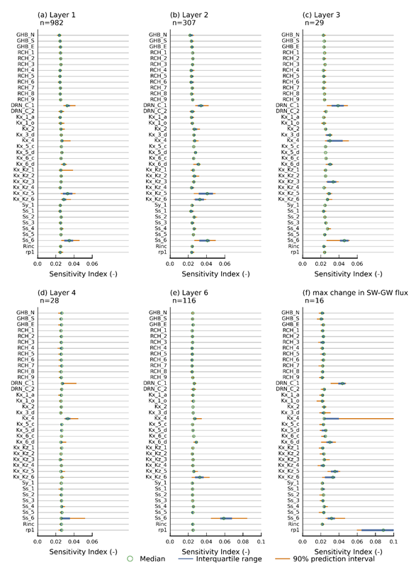
The sensitivity index is a relative metric, high values indicate sensitive parameters, low values indicate less sensitive parameters.
Additional drawdown is dmax, the maximum difference in drawdown between the coal resource development pathway and baseline, due to additional coal resource development.
Source: Gilfedder et al. (2016)
