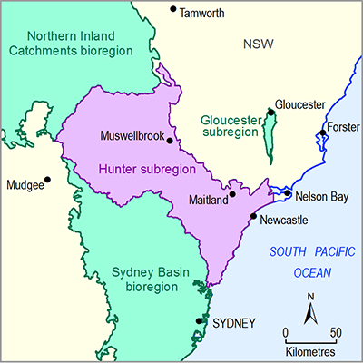
Experts at the Hunter qualitative modelling workshop determined that, given the state of knowledge, wet and dry sclerophyll forests were sufficiently similar in their ecological interactions between the main components and the environment (including groundwater needs) that they could be dealt with in a single model. There were 18.8 km2 of combined wet and dry sclerophyll forests within the zone of potential hydrological change in the Hunter subregion. Landscape class descriptions are given in Table 5 of companion product 2.3 for the Hunter subregion (Dawes et al., 2018). Wet sclerophyll forests are dominated by trees of the Myrtaceae family, particularly of the genera Eucalyptus, Angophora, Corymbia, Syncarpia and Lophostemon. Dominant tree species tend to have smaller, hard leaves and be adapted to varying extents to the occurrence of wild fires. Wet sclerophyll forests are restricted to areas of higher rainfall and moderate fertility and often include a dense understorey of soft-leaved rainforest shrubs and small trees in moister situations (shrubby subformation). In drier situations these forests may have an open, grassy understorey (grassy subformation) with a sparse, sclerophyllous shrub layer. Dry sclerophyll forests are open forests that include a wide range of structural and floristic types. In general they occur on poorer substrates and relatively drier situations than the wet sclerophyll forests. On moderately poor soils these forests may develop a dense, grassy understorey with a more open shrub layer (shrub/grass subformation) while on the poorest substrates (sands and sandstones) a dense, sclerophyllous shrub layer dominates. Fire often plays an important role in the ecology of these forests.
Within the zone of potential hydrological change in the Hunter subregion, dry sclerophyll forests are overwhelmingly dominated by the Keith (2004) vegetation class ‘Sydney coastal dry sclerophyll forests’ (11.9 km2), which are 10- to 25-m tall dry open eucalypt forests with a prominent and diverse sclerophyll shrub understorey and open groundcover of sclerophyll sedges. They occur in areas receiving 1000 mm to over 1300 mm mean annual rainfall, at elevations below 700 m, on quartzose sandstone ridges, slopes and gullies with infertile sandy loams. Common overstorey species are Angophora costata (Sydney red gum) and Corymbia gummifera (red bloodwood) (OEH, 2017b).
Within the zone of potential hydrological change in the Hunter subregion, wet sclerophyll forests are overwhelmingly dominated by the Keith (2004) vegetation class ‘North coast wet sclerophyll forests’ (4.3 km2), which have a subdominant stratum of mesophyllous small trees or tall shrubs up to 15 m tall and a second understorey layer of mesophyllous shrubs above a continuous ground stratum of ferns and herbs. Vines are also present on shrubs and smaller trees. They occur both in coastal ranges and foothills, and on alluvium in sheltered creek flats. They grade into both northern hinterland forests (with decreasing shelter or moisture) and subtropical rainforests (with increasing shelter, moisture or fertility). Dominant canopy species include Eucalyptus acmenioides (white mahogany), E. microcorys (tallowwood), E. pilularis (blackbutt), E. saligna (Sydney blue gum), Lophostemon confertus (brush box) and Syncarpia glomulifera (turpentine) which occur in various combinations in the canopy (OEH, 2017c).
2.7.4.3.1 Qualitative mathematical model
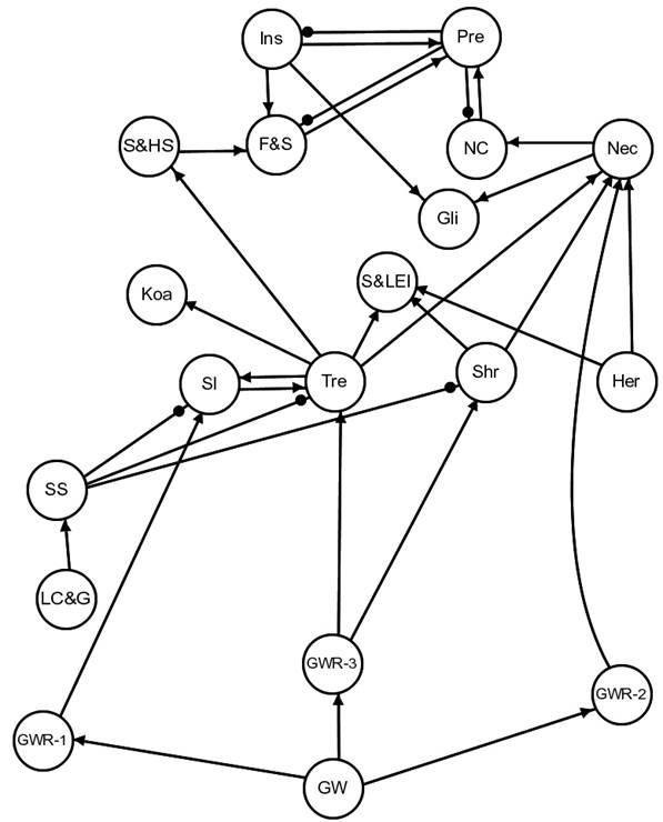
The wet and dry sclerophyll forests signed digraph in Figure 25 is a modified version of the forested wetlands signed digraph. This model lacks life-stage variables for Casuarina spp. and related model variables (i.e. glossy black-cockatoo (GBC), orchids and fungi (O&F), disturbance of leaf litter (Dis)) and components that require a connection with stream or riparian areas (i.e. bank stability (SBS), stream morphology (SM) and wombats (Wom)). Added to this model were variables for populations of koalas (Koa), which use the tree canopy (Tre) for habitat and food resources, and gliders (Gli), which feed on nectar (Nec) and insects (Ins). The same three groundwater regimes identified in the forested wetlands qualitative model were described as being applicable to this system, but the requirement for no permanent inundation (GWR1) over a two-to-three-year period was not relevant to seedlings of non-casuarina tree species because these landscape classes are rarely associated with floodplains and commonly associated with ranges, foothills, ridges, slopes and gullies.
Figure 25 Signed digraph of wet and dry sclerophyll forests
Frogs and skinks (F&S), gliders (Gli), groundwater regime 1 (for seedling ecohydrology) (GWR-1), ground-water regime 2 (for nectar production) (GWR-2), groundwater regime 3 (for tree and shrub canopy cover) (GWR-3), herbs (Her), insects (Ins), koala (Koa), land clearing and grazing (LC&G), nectar consumers (NC), nectar (Nec), predators (Pre), shade and habitat structure (S&HS), sap- and leaf-eating insects (S&LEI), shrubs (Shr), seedling (SI), saline soils (SS), tree (Tre). Hydrological variable added subsequent to the qualitative modelling workshop is groundwater (GW).
Data: Bioregional Assessment Programme (Dataset 2)
In the qualitative models for this landscape class, a decrease in groundwater levels was described as having a negative impact on each of the three groundwater regimes, and a single cumulative impact scenario was developed for qualitative analyses of response predictions. Qualitative analysis of the signed digraph model (Figure 25 and Table 26) generally indicates a negative predicted response for trees (Tre), seedlings (SI) and shrubs (Shr) to the cumulative impact scenario, with a corresponding decline in shade and habitat structure (S&HS), nectar (Nec), nectar consumers (NC), predators (Pre), sap- and leaf-eating insects (S&LEI), gliders (Gli) and koalas (Koa). Insects (Ins) were predicted to increase as a consequence of a release from predation pressure, while no change was predicted for saline soils (SS) and herbs (Her).
Table 26 Predicted response of the signed digraph variables of wet and dry sclerophyll forests to (cumulative) changes in hydrological responses variables
Qualitative model predictions that are completely determined are shown without parentheses. Predictions that are ambiguous but with a high probability (0.80 or greater) of sign determinancy are shown with parentheses. Predictions with a low probability (less than 0.80) of sign determinancy are denoted by a question mark. Zero denotes a completely determined prediction of no change.
Data: Bioregional Assessment Programme (Dataset 2)
2.7.4.3.2 Temporal scope, hydrological response variables and receptor impact variables
The temporal scope for the wet and dry sclerophyll forests is the same as that described for the other landscape classes of the Hunter subregion. For surface water and groundwater variables the reference assessment interval is defined as the 30 years preceding 2012 (i.e. 1983 to 2012). For surface water variables, the short-assessment interval is defined as the 30 years preceding the short-assessment year (i.e. 2013 to 2042), and similarly the long-assessment interval is defined as the 30 years that precede the long-assessment year (i.e. 2073 to 2102). For groundwater, maximum drawdown (metres) and time to maximum drawdown are considered across the full 90-year window: 2013 to 2102.
For wet and dry sclerophyll forests, the qualitative modelling workshop identified one variable –groundwater– as the key hydrological factor governing the quality of the wet and dry sclerophyll forests ecosystem.
As before, this hydrological variable was interpreted as two hydrological response variables that can be modelled (Table 27), and the receptor impact variable formally defined during the receptor impact modelling workshop. As a result, the relationships identified in the qualitative modelling workshop were formalised into a receptor impact model that described the response of:
Table 27 Summary of the hydrological response variables used in the receptor impact models, together with the signed digraph variables that they correspond to, for the wet and dry sclerophyll forests landscape classes in the Hunter subregion
2.7.4.3.3 Receptor impact models
2.7.4.3.3.1 Projected foliage cover of trees
Elicitation scenarios
Table 28 summarises the elicitation design matrix for the projected foliage cover of trees in the ‘Wet sclerophyll forest’ and Dry sclerophyll forest’ landscape classes. The first design point – design point identifier Ref – set the variability in projected foliage cover under the reference conditions (no drawdown).
The remaining design points represent hydrological scenarios that span the uncertainty in the values of the hydrological response variables in the relevant time period of hydrological history associated with the short (2042) and long (2012) assessment years.
Design point identifiers 2 through to 32 (as listed in Table 28) represent combinations of the two hydrological response variables (dmaxRef, tmaxRef), together with high and low values of Yref. The high and low values for Yref were calculated during the receptor impact modelling workshop following the experts’ response to the first design point, and then automatically included within the design for the elicitations at the subsequent design points.
Table 28 Elicitation design matrix for the receptor impact model of mean projected foliage cover in the casuarina tree community in the wet and dry sclerophyll forests landscape classes for the Hunter subregion
Design points for Yref in the future (short- and long-assessment periods) are calculated during the receptor impact model elicitation workshop using elicited values for the receptor impact variable in the reference period. All other design points (with identifiers) are either default values or values determined by groundwater and surface water modelling. Hydrological response variables dmaxRef and tmaxRef are defined in Table 27.
na = not applicable
Data: Bioregional Assessment Programme (Dataset 2)
Receptor impact model
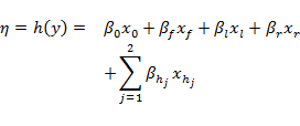
The model fitted to the elicited values of mean percentage foliage cover for the wet and dry sclerophyll forests landscape classes takes the form
|
|
(6) |
where ![]() is an intercept term (a vector of ones),
is an intercept term (a vector of ones), ![]() is a binary indicator variable scored 1 for the case of an assessment in the short- or long-assessment year,
is a binary indicator variable scored 1 for the case of an assessment in the short- or long-assessment year,![]() is a binary indicator variable scored 1 for the case of an assessment in the long-assessment year,
is a binary indicator variable scored 1 for the case of an assessment in the long-assessment year, ![]() is a continuous variable that represent the value of the receptor impact variable in the reference year (Yref, set to zero for the case of an assessment in the reference year), and
is a continuous variable that represent the value of the receptor impact variable in the reference year (Yref, set to zero for the case of an assessment in the reference year), and ![]() are the (continuous or integer) values of the two hydrological response variables (dmaxRef, tmaxRef). Each term has a fitted coefficient
are the (continuous or integer) values of the two hydrological response variables (dmaxRef, tmaxRef). Each term has a fitted coefficient ![]() Note that the modelling framework provides for more complex models, including the quadratic value of, and in interactions between, the hydrological response variables but in this instance the simple linear model above was identified as the most parsimonious representation of the experts’ responses.
Note that the modelling framework provides for more complex models, including the quadratic value of, and in interactions between, the hydrological response variables but in this instance the simple linear model above was identified as the most parsimonious representation of the experts’ responses.
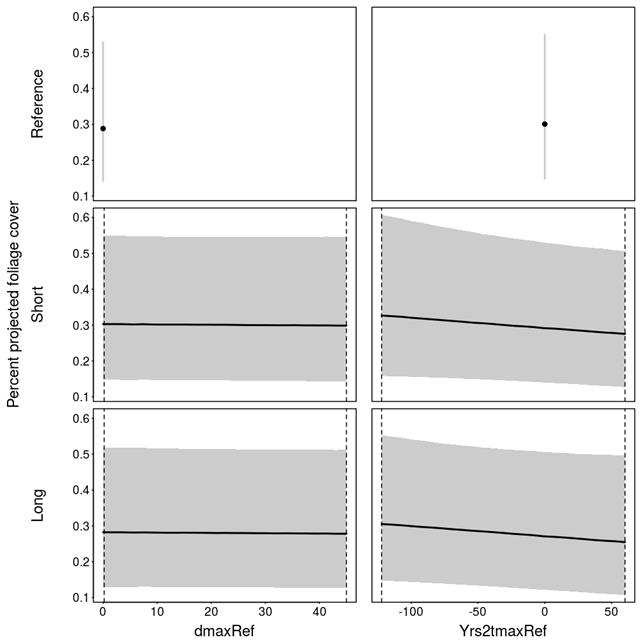
The (marginal) mean and 80% central credible intervals of the two hydrological response variable coefficients are summarised in partial regression plots in Figure 26, whilst Table 29 summarises the same information for all six model coefficients.
In the middle and bottom rows, all other hydrological response variables are held constant at the midpoint of their elicitation range (during risk estimation all hydrological response variables vary simultaneously). Dashed vertical lines show the hydrological response variable range used in the elicitation. dmaxRef is defined in Table 27. Yrs2tmaxRef is the difference between tmaxRef and the assessment year that is relevant for the prediction (2012, 2042 or 2102). The numbers on the y-axis range from 0 to 1 as the receptor impact model was constructed using the proportion for the statistical modelling. They should be interpreted as a percent foliage cover ranging from 0 to 100%.
Data: Bioregional Assessment Programme (Dataset 2)
Table 29 Mean, 10th and 90th percentile of the coefficients of the receptor impact model for projected foliage cover
|
Mean |
q10 |
q90 |
|
|---|---|---|---|
|
(Intercept) |
–1.07 |
–1.86 |
–0.282 |
|
Yref |
1.01 |
0.732 |
1.29 |
|
future1 |
1.08 |
0.253 |
1.91 |
|
long1 |
–0.0999 |
–0.375 |
0.175 |
|
dmaxRef |
–0.000415 |
-0.00474 |
0.00391 |
|
Yrs2tmaxRef |
–0.00129 |
-0.0037 |
0.00112 |
Yref is value of receptor impact variable in the reference assessment year; it has no value if the design case is in the reference assessment year. Future is a binary variable scored 1 if the design case is in a short- or long-assessment year. Long is a binary variable scored 1 if the design case is in the long assessment year. dmaxRef is defined in Table 27. Yrs2tmaxRef is the difference between tmaxRef and the assessment year that is relevant for the prediction (2012, 2042 or 2102).
Data: Bioregional Assessment Programme (Dataset 2)
The model reflects the experts’ opinion that the projected foliage cover in the reference year (Yref) has a positive effect on projected foliage cover in the future. That is, for the same changes in hydrology, a site with a high foliage cover on average in 2012 is likely to have a higher foliage cover on average in the future than a site with a low foliage cover in 2012. This reflects the lag in the response of canopy cover to changes in hydrological response variables that would be expected of mature trees with long life spans.
The model also reflects the experts’ opinion that groundwater drawdown (as indicated by dmaxRef) has a negative effect on average projected foliage cover. In other words, projected foliage cover will decrease as groundwater drawdown increases due to coal resource development. The model predicts that (holding all other hydrological response variables constant at the mid-point of their elicitation range) the mean projected foliage cover will drop from about 32% to about 28% if the groundwater levels decrease by 40 m relative to the reference level in 2012. There is, however, considerable uncertainty in these predictions, with an 80% chance that the canopy cover will lie somewhere between approximately 55% and 15% on the short-assessment period, and somewhere between roughly 52% and 13% in the long-assessment period, with a 40-m drop in groundwater level.
As in the forested wetland model, the mean negative coefficient associated with the covariate Yrs2tmaxRef suggests that projected foliage cover is expected to be higher in the assessment year if the assessment year occurs after the time of maximum drawdown (Yrs2tmaxRef<0 in Figure 26). One interpretation is that the more time that has elapsed since tmaxRef, the greater the groundwater recovery and, in turn, the greater the projected foliage cover in the assessment year. Again, there is considerable uncertainty around the predicted effect on percent projected foliage cover, reflecting uncertainty around the magnitude of and rate at which groundwater levels decline due to pumping and the trees’ ability to adjust to these changes. This is reflected in the large credible intervals in Figure 26.
Finally, the model suggests that we can expect differences in projected foliage cover in the future compared to the reference period, and even between short-term and long-term assessment. While ‘future’ is associated with a positive coefficient, ‘long’ is estimated to have a negative effect on projected foliage cover. This indicates that greater effects are expected in the short-term period than in the long term, as can be observed in Figure 26.

Product Finalisation date
- 2.7.1 Methods
- 2.7.2 Prioritising landscape classes for receptor impact modelling
- 2.7.3 'Riverine' landscape group
- 2.7.4 'Groundwater-dependent ecosystem' landscape group
- 2.7.5 'Coastal lakes and estuaries' landscape group
- 2.7.6 Limitations and gaps
- Citation
- Acknowledgements
- Contributors to the Technical Programme
- About this technical product


