The aim of the quantitative uncertainty analysis is to provide probabilistic estimates of the changes in the hydrological response variables due to coal resource development. A large number of parameter combinations are evaluated and, in line with the Approximate Bayesian Computation outlined in companion submethodology M09 (as listed in Table 1) for propagating uncertainty through models (Peeters et al., 2016), only those parameter combinations that result in acceptable model behaviour are accepted in the parameter ensemble used to make predictions.
Acceptable model behaviour is defined for each hydrological response variable based on the capability of the model to reproduce historical, observed time series of the hydrological response variable. For each hydrological response variable, a goodness of fit between model simulated and observed annual hydrological response variable, as well as an acceptance threshold, are defined.
The ensemble represents the changes in hydrological response variables simulated with the parameter combinations for which the goodness of fit exceeds the acceptance threshold. The resulting ensembles are presented and discussed in Section 2.6.1.6.
Parameter sampling
The parameters included in the uncertainty analysis are the same as those used in the calibration, with the exception that the parameter ne_scale (scaling factor for effective porosity (dimensionless)) is included in the uncertainty analysis. This is because the effective porosity parameter only affects the deep groundwater flow component in the Australian Water Resources Assessment (AWRA) landscape model (AWRA-L). It is unlikely that the calibration is able to uniquely estimate that parameter from the streamflow record, therefore it was not included in the calibration. Its effect on predictions, however, is not clear a priori, which warranted inclusion in the uncertainty analysis.
Table 11 lists the parameters used in the uncertainty analysis and the range sampled in the design of experiment. The sampling within this range is not uniform but is based on a beta distribution biased towards the mean values of the two model calibrations. The AWRA-L and AWRA river model (AWRA-R) parameters in Table 11 are explained in the AWRA-L v4.5 documentation (Viney et al., 2015) and AWRA-R v5.0 documentation (Dutta et al., 2015), respectively. Parameters with a large order of magnitude range in parameter bounds, or that are thought to be particularly sensitive to low parameter values, are transformed logarithmically to ensure that values near the minimum of the range are adequately sampled.
Table 11 Summary of AWRA-L and AWRA-R parameters for uncertainty analysis
AWRA-L = Australian Water Resources Assessment landscape model; AWRA-R = Australian Water Resources Assessment river model; na = data not applicable, Kg = groundwater drainage coefficient (d-1), Kr = rate coefficient controlling discharge to stream (dimensionless), Ksat = saturated hydraulic conductivity (mm d-1), Pref = reference precipitation
Three thousand parameter combinations are generated from the AWRA-L and AWRA-R model parameters according to the ranges and transformations shown in Table 11. These ranges and transformations are chosen by the modelling team based on previous experience in regional and continental calibration of AWRA-L (Vaze et al., 2013) and AWRA-R (Dutta et al., 2015). These mostly correspond to the upper and lower limits of each parameter that are applied during calibration.
The parameter combinations are generated together with the parameter combinations for the groundwater model (see companion product 2.6.2 for the Namoi subregion (Janardhanan et al., 2018)). This linking of parameter combinations allows the results to consistently propagate from one model to another, as outlined in the model sequence section (Section 2.6.1.1).
Each of the 3000 parameter sets is used to drive AWRA-L to generate a runoff time series at each 0.05 x 0.05 degree (~5 x 5 km) grid cell. The resulting runoff is accumulated to the scale of the AWRA-R subcatchments and is used – in conjunction with the sampled AWRA-R parameters – to drive AWRA-R.
Observations
Predictions and observations from 32 streamflow gauges of catchments which contribute flow to the surface water modelling domain in the Namoi subregion are used for uncertainty analysis. Selection of the 32 streamflow gauges is based on three criteria: (i) data length more than 10 years, (ii) not subject to major open-cut and underground mine impacts, and (iii) not subject to major dam control. For these streamflow gauges, historical observations of streamflow are summarised into the nine hydrological response variables for all years. The equivalent simulated hydrological response variable values are computed from the 3000 design of experiment runs. The goodness of fit between these observed and simulated hydrological response variable values is used to constrain the 3000 parameter combinations and select the best 10% of replicates (i.e. 300 replicates) for each hydrological response variable. Predictions from these 300 replicates are reported in Section 2.6.1.6.
Predictions
For each of the 54 model nodes the post-processing of design of experiment results in 3000 time series with a length of 90 years (2013 to 2102) of hydrological response variable values for baseline (![]() ) and CRDP conditions (
) and CRDP conditions (![]() .
.
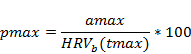
These time series for baseline and CRDP are summarised through the maximum raw change (amax), the maximum percent change (pmax) and the year of maximum change (tmax). The percent change is defined as:
|
|
(1) |
As the predictions include the effect of surface water – groundwater interaction through coupling with the groundwater models, it is possible that the groundwater parameters affect the surface water predictions.
Selection of parameter combinations
The acceptance threshold for each hydrological response variable is set to the 90th percentile of the average goodness of fit between observed and simulated hydrological response variable values obtained from model nodes at 32 streamflow gauging sites. This means that out of the 3000 model replicates, the 300 best (10%) are selected for each hydrological response variable.
The selection of the 10% threshold is based on two considerations: (i) guaranteeing enough prediction samples to ensure numerical robustness, and (ii) the sample’s prediction performance is close to that obtained from the high- and low-streamflow model calibrations. Furthermore, it is expected that the full 3000 replicates contain many with infeasible parameter combinations (caused, for example, by parameter correlations that are not considered in the independent random sampling) and that these are likely to be filtered out by sampling only the best 10% of replicates. Nevertheless, selecting the best 10% of replicates is determined arbitrarily, and the implications of this decision are further discussed in Section 2.6.1.5.2.
