Data
Input data to drive the AWRA river model (AWRA-R) calibration include climate, potential evaporation, catchment runoff (from AWRA-L), groundwater depth, and power generation and town water supply diversions. Calibration datasets against which performance of AWRA-R and the various modules were evaluated are daily streamflow, dam storage volumes, water allocations, dam releases and irrigation diversions.
The calibration period for the different AWRA-R components generally covered 1981 to 2012. However, some calibration datasets did not cover this entire period and suitable periods were chosen based on data availability; details of these datasets are provided below.
The only direct climate input into AWRA-R is daily precipitation, which is used to calculate precipitation directly on the river channel and storages. Daily gridded precipitation data from the Bureau of Meteorology (Dataset 1) have been used in the calibration of AWRA-R. The gridded data were clipped and aggregated (spatially averaged) using reach subcatchment boundaries defined in the Hunter river system AWRA-R node-link network (Bioregional Assessment Programme, Dataset 7 and Dataset 8).
Daily estimates of potential evaporation and catchment runoff were obtained from the calibrated AWRA-L simulation (Bioregional Assessment Programme, Dataset 6) and aggregated to the reach scale defined by the Hunter river system node-link network (Bioregional Assessment Programme, Dataset 7 and Dataset 8) for input into AWRA-R.
Industry diversions (including those for power stations and town water supply) are not calibrated and are used as inputs in AWRA-R (NSW Office of Water, Dataset 9).
The AWRA-R model used for calibration comprises 52 nodes and their contributing areas, shown in Figure 11. These include the 34 gauging stations for which stage and streamflow data were obtained for model calibration (Bureau of Meteorology, Dataset 5). Twenty of the gauging stations are non-headwater gauges: they include 11 on the Hunter River, three on each of Wollombi Brook and the Goulburn River and three on other Hunter River tributaries (red triangles in Figure 11). The other 32 calibration model nodes (black dots in Figure 11) comprise the 14 gauging stations on headwater streams, plus 18 of the 29 model nodes (see Section 2.6.1.3.2), located on ungauged headwater streams. Daily streamflows at the 18 ungauged nodes are simulated by AWRA-L (Bioregional Assessment Programme, Dataset 6) and stages obtained from idealised cross-sections at each location (see companion product 2.1-2.2 for the Hunter subregion (Herron et al., 2018); Bioregional Assessment Programme, Dataset 10). Eleven model nodes, located on ungauged reaches downstream of other model nodes, are not used in the calibration but are needed for the AWRA-R model simulations.
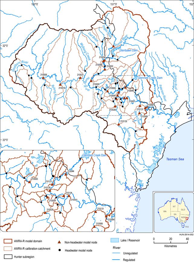
AWRA-R = Australian Water Resources Assessment river model
Data: Bureau of Meteorology (Dataset 5), Bioregional Assessment Programme (Dataset 7, Dataset 8)
Daily irrigation and mining diversions were sourced from the Hunter Integrated Quantity-Quality Model (IQQM) (NSW Office of Water, Dataset 9), aggregated to monthly for the period 1981 to 2012. Irrigation diversions were used to calibrate the AWRA-R irrigation and dam storage and releases modules. Mining diversions were used as inputs in the calibration. Since mining diversions have similar seasonal patterns to irrigation diversions, the AWRA-R irrigation module is used to simulate mining diversions under baseline and CRDP.
Available observed stored volumes as well as allocations (NSW Office of Water, Dataset 9) were used in preference to simulated data for calibration of the dam storage module. These data were available from 1993 to 2012.
Daily dam releases (for Glenbawn Dam and Glennies Creek Dam) were sourced from the Hunter IQQM (NSW Office of Water, Dataset 9). These data were available from 1981 to 2012.
All data used for calibration of allocation, dam storage and dam releases overlapped the period from 1993 to 2012, hence this period was chosen for calibration of these components.
Model calibration results
Streamflow routing and reach water balance
AWRA-R was calibrated using 34 streamflow gauges defining a concurrent number of modelling reaches. Two variants of the model were calibrated using AWRA-L high-streamflow and low-streamflow calibration outputs, respectively (Bioregional Assessment Programme, Dataset 6). Eight of the 11 AWRA-R parameters (Viney, 2016) were calibrated; one routing parameter was fixed and the floodplain module (two parameters) was not implemented. The parameter values for the two calibrations are included in Bioregional Assessment Programme (Dataset 6).
The agreement of both high- and low-streamflow AWRA-R calibrations were assessed using the daily Nash–Sutcliffe efficiency (Ed) for daily streamflow (Ed(1.0)) and for daily streamflow transformed with a Box-Cox lambda value of 0.1 (Ed(0.1)) as well as both F1 and F2 values (see Section 2.6.1.4.1). The bias generally remains very low as each reach is individually calibrated and parameterised, as opposed to the regional calibration implemented for AWRA-L (see companion submethodology M06 (as listed in Table 1) for surface water modelling (Viney, 2016)).
The performance is reported for the 20 non-headwater gauges depicted as triangles in Figure 11 and where routing and reach water balance processes (including runoff from catchments between the two nodes, river water diversions, groundwater fluxes and overbank flow) take place.
Figure 12 shows boxplots summarising the performance of the AWRA-R high-streamflow and AWRA-R low-streamflow calibrations in the 20 gauges. Table 7 presents a summary of the goodness-of-fit metrics used to evaluate the two model variants. In terms of Ed(1.0) (emphasis on high flows), the AWRA-R high-streamflow calibration agrees reasonably well with observations, indicated by a median Ed(1.0) of 0.73 (interquartile range of 0.53 to 0.79) and a median bias of 0.005. Thirteen of the 20 reaches have an Ed(1.0) greater than 0.6, whereas only reach 210006 (Goulburn River at Coggan) has an Ed(1.0) less than 0.25.
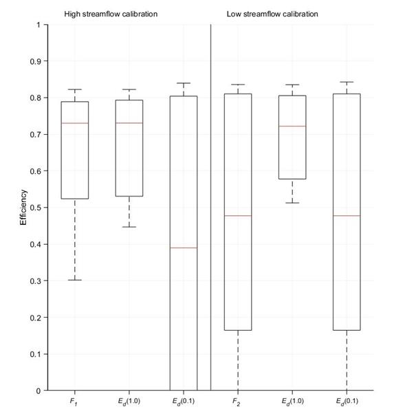
Figure 12 Summary of two AWRA-R model calibrations for the Hunter River
AWRA-R = Australian Water Resources Assessment river model
In each boxplot, the bottom, middle and top of the box are the 25th, 50th and 75th percentiles, and the bottom and top whiskers are the 10th and 90th percentiles. F1 is the F value for high-streamflow calibration; F2 is the F value for the low-streamflow calibration; Ed(1.0) is the daily efficiency with a Box-Cox lambda value of 1.0; Ed(0.1) is the daily efficiency with a Box-Cox lambda value of 0.1.
Data: Bioregional Assessment Programme (Dataset 6)
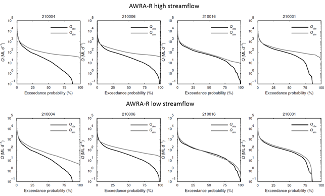
Overall agreement in terms of Ed(0.1) (emphasis on medium to low flows) for the AWRA-R high-streamflow calibration is poorer than Ed(1.0), with a median value of 0.39 (interquartile range of 0.15 to 0.80). Eight of the 20 reaches have an Ed(0.1) greater than 0.5. Low Ed(0.1) values (<0.3) are observed in some reaches in the Goulburn River and Wollombi Brook, where the intermittent nature of streamflow is not captured by the model. This is highlighted in the flow duration curves for gauging stations in both Wollombi Brook and Goulburn River (Figure 13). The high-streamflow calibration yields a median F1 of 0.52 and median bias is about 0.005. It should be noted that no Goulburn River catchments were included in the regional AWRA-L calibration as they were impacted by coal mining developments and did not meet the criteria for inclusion (see Section 2.6.1.4.1 and Figure 8).
The overall results in the 20 main calibration gauges are generally better than those obtained at other river basins across Australia (Dutta et al., 2015).
AWRA-R = Australian Water Resources Assessment river model
Data: Bioregional Assessment Programme (Dataset 6)
The AWRA-R low-streamflow calibration has a median Ed(1.0) of 0.72 (interquartile range of 0.58 to 0.81). Fourteen out of the 20 reaches have an Ed(1.0) greater than 0.6 and, again, only reach 210006 (Goulburn River at Coggan) has an Ed(1.0) value less than 0.49. In terms of Ed(0.1) for AWRA-R low-streamflow calibration, model performance is markedly better than for the AWRA-R high-streamflow calibration, with a median value of 0.48 (interquartile range of 0.16 to 0.81). Only eight reaches have an Ed(0.1) greater than 0.6. The performance in the reaches in the Goulburn River and Wollombi Brook improve remarkably with the six reaches in those streams having a median Ed(0.1) of 0.38 for AWRA-R low-streamflow calibration, compared to a median Ed(0.1) of 0.05 for AWRA-R high-streamflow calibration. As a result the model agrees better with medium to low streamflow and the intermittent nature of streamflow at some of these gauging stations. This is particularly evident in the flow duration curves for 210016 and 210031 shown in Figure 13 for high- and low-streamflow calibrations. The low-streamflow calibration has a median F2 value of 0.48 and a median bias of 0.002.
Table 7 Summary of AWRA-R calibration for the 20 reaches in the Hunter subregion
AWRA-R = Australian Water Resources Assessment river model; F1 = F value for high-streamflow calibration; F2 = F value for low-streamflow calibration (see Viney, 2016); Ed(1.0) = daily efficiency with a Box-Cox lambda value of 1.0; Ed(0.1) = daily efficiency with a Box-Cox lambda value of 0.1
Data: Bioregional Assessment Programme (Dataset 6)
The impact of including seven additional reaches on the calibration of AWRA-R generally degrades agreement with observations in the reaches immediately downstream of these reaches. For example, the median Ed(1.0) using the high-streamflow calibration with the additional reaches is 0.66 (range 0.12 to 0.88). The largest degradation is for the Hunter River at Denman (210055), where Ed(1.0) decreases from 0.79 to 0.59, followed by Wollombi Brook at Bulga (210028) (0.77 to 0.63) and Hunter River at Liddell (210083) (0.81 to 0.67). Changes in Ed(1.0) are marginal (<0.05) in the rest of the gauging stations. Again, median bias is less than 0.005.
Boxplots in Figure 14 show the bias of the two calibration schemes (AWRA-R high-streamflow and AWRA-R low-streamflow calibration) in predicting the nine hydrological response variables that characterise the impacts of coal resource development on water resources (see Section 2.6.1.4.1). Similar to the AWRA-L results, these boxplots show that generally the AWRA-R low-streamflow calibration has smaller model biases and narrower interquartile ranges than the AWRA-R high-streamflow calibration for the low-streamflow metrics (LFD, LFS, LLFS and P01). ZFD remains poorly simulated. The median biases in the high-streamflow metrics are generally marginally smaller in the high-streamflow calibration, and the interquartile ranges are narrower, highlighting less variability among the hydrological response variables in the calibrated Hunter reaches.
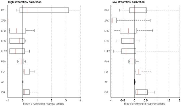
AWRA-R = Australian Water Resources Assessment river model
In each boxplot, the left, middle and right of the box are the 25th, 50th and 75th percentiles, and the left and right whiskers are the 10th and 90th percentiles for the 20 AWRA-R calibration reaches.
Shortened forms of hydrological response variables are defined in Table 6.
Data: Bioregional Assessment Programme (Dataset 6)
Irrigation module
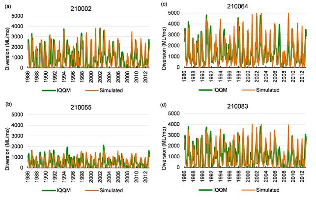
The irrigation module in AWRA-R was calibrated in nine reaches along the Hunter River and one reach of Glennies Creek (210044). Calibration was performed against monthly IQQM simulated diversions for the period 1986 to 2012 using allocation data (NSW Office of Water, Dataset 9) and AWRA-R simulated streamflow (Bioregional Assessment Programme, Dataset 6). Details of the land use dataset and how it was used to parameterise the irrigation module are provided in companion product 2.1-2.2 for the Hunter subregion (Herron et al., 2018).
Table 8 presents a summary of goodness-of-fit metrics used to evaluate the performance of calibration. Simulated and observed diversions were compared using the (i) coefficient of determination (r2), which indicates the agreement in temporal patterns, (ii) monthly Nash–Sutcliffe efficiency (Em), which indicates the calibration accuracy, and (iii) bias (B), which indicates the overall tendency of the model towards overestimation or underestimation. Good diversion patterns were simulated in all reaches, with a median r2 of 0.82 (range 0.71 to 0.91).
Table 8 Summary of AWRA-R irrigation calibration for nine reaches in the Hunter subregion
AWRA-R = Australian Water Resources Assessment river model; r2 = coefficient of determination; Em = monthly Nash–Sutcliffe efficiency; B = model bias
Data: Bioregional Assessment Programme (Dataset 6), NSW Office of Water (Dataset 9)
Figure 15 shows time series of observed and simulated diversions for the four reaches of the Hunter River with the highest water use. Inter-annual and intra-annual variability are generally captured by the model, with a mean Em of 0.67 (range 0.43 to 0.79).
The variance in Em is greater than the variance in r2 (Table 8), indicating model overestimation or underestimation (van Dijk et al., 2008). Diversions are under estimated in five reaches, but the underestimation only exceeds 10% in reach 210044. The mean absolute bias in all reaches is 0.04.
Dam storage volumes, releases and allocations
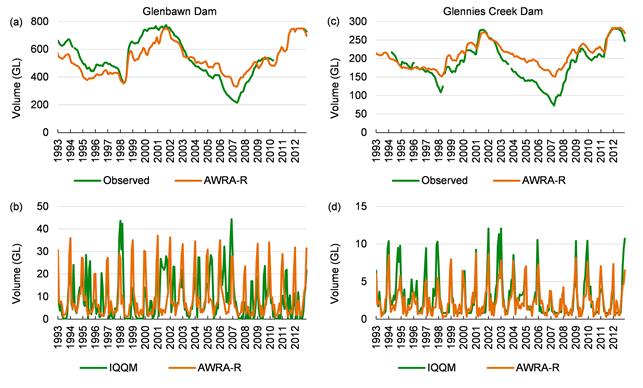
Storage volumes for Glenbawn Dam and Glennies Creek Dam, releases and allocations were calibrated as a whole system against observed daily storage volumes and IQQM simulated releases (NSW Office of Water, Dataset 9). Individual dam volumes and releases were subsequently estimated from the allocations and a split value based on IQQM simulated releases. The calibration methodology and justification is described in companion submethodology M06 (as listed in Table 1) for surface water modelling (Viney, 2016).
Goodness-of-fit metrics used to evaluate the performance on calibrated storage volumes and dam releases included the monthly Nash–Sutcliffe efficiency (Em), the coefficient of determination (r2) and the root-mean-square error (RMSE) to assess the overall accuracy.
IQQM = Integrated Quantity-Quality Model
Data: Bioregional Assessment Programme (Dataset 6), NSW Office of Water (Dataset 9)
For illustrative purposes, time series of monthly storage volumes are shown in Figure 16a and Figure 16c. Temporal patterns agree well with observations, with r2 values of 0.87 and 0.89 for Glenbawn Dam and Glennies Creek Dam, respectively. In contrast, modelled volumes are modest for Glenbawn Dam (Em = 0.37) and poor for Glennies Creek Dam (Em = 0.1). The RMSE is 79 GL and 33 GL for Glenbawn Dam and Glennies Creek Dam, respectively, or about 15% of their mean storage volumes. It can be seen in Figure 16 that AWRA-R generally under estimates storage volumes between 1993 and 2002, but over estimates them during the dry period between 2003 and 2008.
Time series of monthly dam releases are shown in Figure 16b and Figure 16d. Temporal patterns agree reasonably well with observations, with r2 values of 0.5 and 0.84 for Glenbawn Dam and Glennies Creek Dam, respectively. Simulated releases are poor for Glenbawn Dam (Em = 0.01) but good for Glennies Creek Dam (Em = 0.65). The RMSE for the calibration period (1993 to 2012) is 9.4 GL and 1.5 GL for Glenbawn Dam and Glennies Creek Dam releases, respectively.
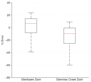
Figure 17 summarises the monthly percentage error (computed as the percentage of the difference between volume simulated and observed divided by simulated volume) for both dams. The error is generally –20% to +20%, which suggests that the modelled allocations will generally be within this margin of error.
AWRA-R = Australian Water Resources Assessment river model; IQQM = Integrated Quantity-Quality Model
Data: Bioregional Assessment Programme (Dataset 6), NSW Office of Water (Dataset 9, Dataset 11)
The poor monthly efficiencies for the simulated releases from Glenbawn Dam can be attributed to the imposed releases in December and January to satisfy water demand for the environment and for electricity generation. Although electricity generation demand does not dominate the variance in the dam releases (r2= 0.15, whereas for irrigation and mine demand r2= 0.27), it drives some of the peak releases, particularly during the dry period of 2003–2008. As a result, the dam model misses some of these peaks (i.e. those occurring in months other than December and January), or simulates greater peaks in December and January. When only irrigation and mining demand are considered, AWRA-R releases can explain 45% of the variance. In the case of Glennies Creek Dam releases, the model conceptualisation captures well the downstream irrigation and mining demand, which comprises about 100% of diversions.
Time series of observed and estimated allocations are shown in Figure 18. Simulated allocations are less than 100% during 1995 to 1999 and during 2006 to 2008. Observed allocations are 100% during 1995 to 1999 despite dam volumes being around 50% full; this may reflect changes in licence volumes and/or policy that are not considered in the model. Allocations are over estimated by the model in the second dry period (2006 to 2008) when dams are at around 30% of their capacity, mainly because differences between simulated and observed dam volumes are about 30% and 50% for Glenbawn Dam and Glennies Creek Dam, respectively.
Data: Bioregional Assessment Programme (Dataset 6), NSW Office of Water (Dataset 9)
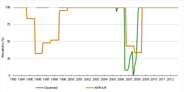
Figure 18 Observed and AWRA-R simulated allocations for the AWRA-R Hunter river system
AWRA-R = Australian Water Resources Assessment river model
Data: Bioregional Assessment Programme (Dataset 6), NSW Office of Water (Dataset 9)
Implications for model predictions
Overall, AWRA-R streamflow is reasonably well simulated using both high- and low-streamflow calibrations. As expected, the low-streamflow calibration performed markedly better when the evaluation was focused on the low flows, particularly in intermittent streams. The better performance of the low-streamflow calibration was also observed in terms of the hydrological response variables used to quantify the hydrological changes due to the additional coal resource development, particularly for the variables characterising low streamflow, although the performance for the variables characterising high flows was typically only marginally worse. Generally, the hydrological response variables characterising low-streamflow conditions are under estimated, whereas those characterising high-streamflow conditions are over estimated. The number of ZFD remains poorly simulated with either model variant, though is slightly better for the low-streamflow calibration.
Similar to AWRA-L calibrations, the parameter sets obtained for AWRA-R high- and low-streamflow calibrations show large uncertainty in predicting the nine hydrological response variables. Prior distributions of the model parameters are used in Approximate Bayesian Computation uncertainty analysis to generate 3000 parameter sets which cover wide boundary ranges for two of the AWRA-R calibration parameters (see Section 2.6.1.5). The outputs from simulations that use the 3000 parameter sets for both AWRA-L and AWRA-R are expected to provide suitable uncertainty bounds for predicting the hydrological changes due to the additional coal resource development on the nine hydrological response variables in each model node in the Hunter subregion (Section 2.6.1.6).
A wide range of dam operating conditions are represented in the model as a result of choosing a 20-year calibration period that included significant dry and wet periods. This ensures that the model can be used in some of the extreme conditions imposed by modelling of the additional coal resource development. The simple soil water deficit that computes releases for irrigation, and the scheme (through a similar deficit proxy) that computes releases for mining perform reasonably well. This is highlighted in the reasonably good agreement (r2 and Em both greater than 0.6) between simulated and IQQM-modelled releases for Glennies Creek Dam, for which irrigation and mining diversions comprise about 100% of surface water diversions; and by Glenbawn Dam releases explaining 45% of the variance when only irrigation and mining demand are considered.
AWRA-R simulated dam storage volumes, releases and allocations are reasonable and comparable to studies that simulated dam volumes and releases in multi-purpose reservoirs for scenario modelling (see Wu and Chen, 2012). Most of the mismatch can be attributed to imposing a pattern of summer dam releases for the environment and for electricity generation (the largest water user in the Hunter river basin) on the model, which does not accurately reflect the actual demand pattern. It is acknowledged that a more robust scheme is needed to simulate releases to satisfy water demand for electricity generation.
Overestimation of releases during the dry period between 2003 and 2008 can be partly explained by high water demand for electricity generation, but also by AWRA-L inflows to both dams, as AWRA-L tends to over estimate streamflow in the Hunter River during this drought period. Moreover, the calibration scheme uses one parameter per dam that linearly scales these inflows, thus it is difficult to solve this issue through calibration of the AWRA-R dam module only. Improvement of model performance can be achieved through better model conceptualisation and calibration strategies.
