Data
Data needed for calibration of the Australian Water Resources Assessment (AWRA) landscape model (AWRA-L) include climate data and streamflow. The calibration period used for AWRA-L model development was from 1983 to 2012, which includes both wet and dry periods.
The landscape water balance model AWRA-L is run using gridded data of maximum temperature, minimum temperature, incoming solar radiation and precipitation. Daily grids (cell resolution of 0.05 x 0.05 degrees; ~5 x 5 km) of these variables are generated for the Australian continent by the Bureau of Meteorology (Dataset 1). Details of this dataset are provided in Section 2.1.1 of companion product 2.1-2.2 for the Hunter subregion (Herron et al., 2018).
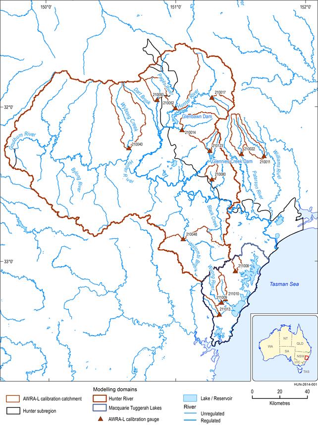
Daily stage and streamflow data from 14 streamflow gauging stations with unregulated catchments located in and near the Hunter subregion were used to calibrate AWRA-L. These gauging stations and the catchments subtended by them are shown in Figure 8. Ten stations are located in the Hunter river basin and four in the Macquarie-Tuggerah lakes basin. Of the 14 stations, ten are located within the modelling domain (Section 2.6.1.3) and four are located very close by. Site details are summarised in Section 2.1.4 of companion product 2.1-2.2 for the Hunter subregion (Herron et al., 2018). Observed daily mean streamflow data for the above gauges for 1983 to 2012 were derived from NSW DPI water data supplied by the Bureau of Meteorology (Dataset 2).
Criteria for selecting the calibration catchments include that they:
- have catchment areas greater than 50 km2
- have long-term measurements (more than 20 years from 1983)
- are currently not impacted by coal mining or coal seam gas extraction or other major extractive industries
- have no significant flow regulation (e.g. dams)
- are not nested (i.e. not directly upstream or downstream of another selected gauge)
- are located within or close to the Hunter subregion and have similar catchment sizes and climate regimes.
Catchment boundaries for the 14 calibration catchments were delineated using the Australian Hydrological Geospatial Fabric (Geofabric) (Bureau of Meteorology, Dataset 5).
AWRA-L = Australian Water Resources Assessment landscape model
Data: Bioregional Assessment Programme (Dataset 3, Dataset 4), Bureau of Meteorology (Dataset 5)
Calibration evaluation metrics
As per companion submethodology M06 (as listed in Table 1) for surface water modelling (Viney, 2016), two regional model calibrations were undertaken: one biased towards predicting high-streamflow behaviour; the second biased towards predicting low-streamflow behaviour. Three metrics were used to evaluate model performance:
- Daily efficiency (Ed), also referred to as the Nash–Sutcliffe efficiency, which compares daily model predictions against daily observation data. Efficiency values range from 1 (which indicates perfect agreement between prediction and observation) to minus infinity.
- Model bias (B), the prediction error divided by the sum of observations, which gives an indication of the model’s overall tendency towards underprediction or overprediction. Bias ranges from –1 (negative values indicate underprediction) to plus infinity (overprediction). The closer the model bias is to zero, the better the model is at estimating the observed volume of streamflow.
- F value, which seeks to combine efficiency and bias into a single metric. The high-streamflow calibration uses a version of F given by F1 = (Ed(1.0) + Em)/2 - 5)|In(1 + B)|2.5, where Ed(1.0) is the efficiency of daily streamflow (without transformation, or with a Box-Cox lambda value of 1.0) (Box and Cox, 1964), Em is the efficiency of the monthly predictions assessed against monthly observations, and B is the bias. The low-streamflow calibration uses a version of F given by F2 = Ed(0.1) - 5)|In(1 + B)|2.5, where Ed(0.1) is the efficiency of daily streamflow transformed with a Box-Cox lambda value of 0.1.
Model calibration results
Figure 9 and Table 5 summarise results of the two model calibrations for the 14 calibration catchments in terms of the three performance metrics. The parameter values for the two calibrations are included in Bioregional Assessment Programme (Dataset 6). The high-streamflow calibration yields a reasonable Nash–Sutcliffe efficiency of daily streamflow, indicated by a median Ed(1.0) of 0.45 and interquartile range of 0.4 to 0.6. Overall model bias is low with a median bias of –0.03, but the interquartile range indicates variability across the 14 catchments with considerable overestimation in some catchments. The high-streamflow calibration yields a median F1 of 0.37, which is only 0.08 less than the median Ed(1.0), indicating overall low model bias. The Ed(1.0) value is negative (suggesting poor simulation) for one catchment: –0.16 at gauging station 211010 on the Wyong River, with a prediction bias of 0.68.
The low-streamflow calibration is evaluated against the daily streamflow data transformed with a Box-Cox lambda value of 0.1. The low-streamflow calibration yields similar efficiency to the high-streamflow calibration, indicated by a median Ed(1.0) of 0.41. The Ed(1.0) is greater than 0.34 for 11 of the 14 catchments and remains above zero for all catchments. The median bias of –0.12 indicates an overall tendency for underprediction by the low-streamflow calibration.
The performance of the high-streamflow calibration for the 14 catchments is not significantly related to catchment wetness, as it does not perform better or worse with a wetter climate. The Ed(0.1) values of the low-streamflow calibration are moderately correlated with catchment wetness (r2 = 0.51, p < 0.01), but the statistical significance of this correlation does not extend to F2.
The 14 calibration catchments cover a wide range of climate and topographic conditions, with mean annual flow (AF) ranging from 33 mm/year at catchment 210040 (Wybong Creek) to 425 mm/year at catchment 210011 (Williams River) (Table 5). This suggests that AWRA-L can predict streamflow variability reasonably in the Hunter subregion where climate conditions vary widely.
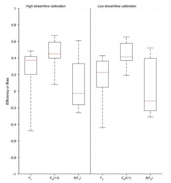
Figure 9 Summary of two AWRA-L model calibrations for the Hunter subregion
AWRA-L = Australian Water Resources Assessment landscape model
In each boxplot, the bottom, middle and top of the box are the 25th, 50th and 75th percentiles, and the bottom and top whiskers are the 10th and 90th percentiles. F1 is the F value for high-streamflow calibration; F2 is the F value for the low-streamflow calibration; Ed(1.0) is the daily efficiency with a Box-Cox lambda value of 1.0; Ed(0.1) is the daily efficiency with a Box-Cox lambda value of 0.1; B is model bias.
Data: Bioregional Assessment Programme (Dataset 6)
Table 5 Calibration statistics for the 14 AWRA-L calibration catchments
AWRA-L = Australian Water Resources Assessment landscape model; F1 = F value for high-streamflow calibration; F2 = F value for low-streamflow calibration (see Viney, 2016); Ed(1.0) = daily efficiency with a Box-Cox lambda value of 1.0; Ed(0.1) = daily efficiency with a Box-Cox lambda value of 0.1
Data: Bioregional Assessment Programme (Dataset 6)
Nine hydrological response variables (Table 6) have been chosen to characterise the hydrological changes of coal resource development on water resources. Figure 10 shows the model bias in the prediction of the hydrological response variables based on the high- and low-streamflow calibrations. Overall, the low-streamflow calibration outperforms the high-streamflow calibration across the nine hydrological response variables with smaller median model biases and narrower interquartile ranges for the 14 catchments. Only for AF does the high-streamflow calibration yield better predictions than the low-streamflow calibration. Both calibrations tend to over estimate both the high-streamflow metrics high-flow days (FD) and interquartile range (IQR), but tend to under estimate daily streamflow at the 99th percentile (P99). Both calibrations tend to under estimate the low-streamflow metrics: low-flow days (LFD), low-flow spells (LFS) and longest low-flow spell (LLFS). The median bias for daily streamflow at the 1st percentile (P01) is close to zero for both calibrations, but some catchments over estimate P01 significantly. Neither calibration predicts zero-flow days (ZFD) well, although for most subcatchments there are very few days in the observed data without flow.
Table 6 Hydrological response variables used to characterise hydrological changes of coal resource development
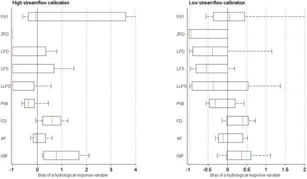
In each boxplot, the left, middle and right of the box are the 25th, 50th and 75th percentiles, and the left and right whiskers are the 10th and 90th percentiles.
Shortened forms of hydrological response variables are defined in Table 6.
Data: Bioregional Assessment Programme (Dataset 6)
It is noted that the parameter sets obtained from the regional model calibrations are not applied directly to the uncertainty analysis (Section 2.6.1.5). However, they are taken as reference values to evaluate performance of the best 10% of parameter sets (i.e. 300 model runs) selected for each hydrological response variable.
Implications for model predictions
Results from the regional model calibrations (Table 5 and Figure 9) suggest that AWRA-L performs reasonably well in estimating high streamflow and low streamflow in the Hunter subregion.
It is noted that when the model is calibrated against observations from 14 streamflow gauges it does not generate a uniform model performance. Though the model performs well overall, it performs poorly in some catchments and does not estimate the suite of hydrological response variables equally effectively. For instance, the high-streamflow model calibration generates a poor model performance at gauge 211010. The model noticeably under estimates streamflow for gauges 211010 and 210048. For other gauges in the Hunter subregion, AWRA-L performs well in terms of model efficiency and bias.
As opposed to model calibration against observation at each individual catchment, a key characteristic of regional model calibration against observations from multiple catchments is that there is no noticeable degradation from model calibration to model prediction (Viney et al., 2014). For both the high- and low-streamflow calibrations, the biases at the majority of individual stream gauging sites are in the range –20% to +40%. Given the regionalisation methodology applied here, it is reasonable to assume that prediction biases in ungauged parts of the subregion will be similar. This provides confidence when applying AWRA-L to each model node where there are no streamflow observations.
The results from the simulated hydrological response variables (Figure 10) show that in the Hunter subregion, AWRA-L calibrated against high daily streamflow is not always better for estimating the high-streamflow hydrological response variables; and the model calibrated against low daily streamflow performs consistently better than that based on the high-streamflow calibration for estimating most hydrological response variables. Both calibrations, however, show large uncertainty in predicting some of the hydrological response variables. In general, one or other of the two calibration sets provides predictions of the hydrological response variables with little bias. An exception is for the variable describing the number of low-flow days, which both parameter sets severely under-predict. This suggests that less confidence may be ascribed to the prediction of this variable in Section 2.6.1.6 than to the prediction of the other variables. Using both calibration parameter sets to generate the 3000 parameter sets for the simulations is expected to provide a reasonable estimate of uncertainty for each hydrological response variable.
