2.7.4.1.1 Description
This section describes and presents ecological modelling for the ‘Non-floodplain or upland riverine’ landscape group for the non-Pilliga regions in the zone of potential hydrological change of the Namoi subregion. This landscape group encompasses the riverine habitat, adjacent riparian areas and remnant patches of vegetation across different positions in the landscape classed as ‘Grassy woodland GDE’ (Figure 15). The upland environment includes the following riverine classes:
- ‘Permanent upland stream’
- ‘Permanent upland stream GDE’
- ‘Temporary upland stream’
- ‘Temporary upland stream GDE’.

Some key landscape classes are labelled including: ‘Temporary upland stream GDE’, ‘Upland riparian forest GDE’ and ‘Grassy woodland’ (non- water-dependent).
GDE = groundwater-dependent ecosystem
Source: Symbols courtesy of the Integration and Application Network (ian.umces.edu/symbols/)
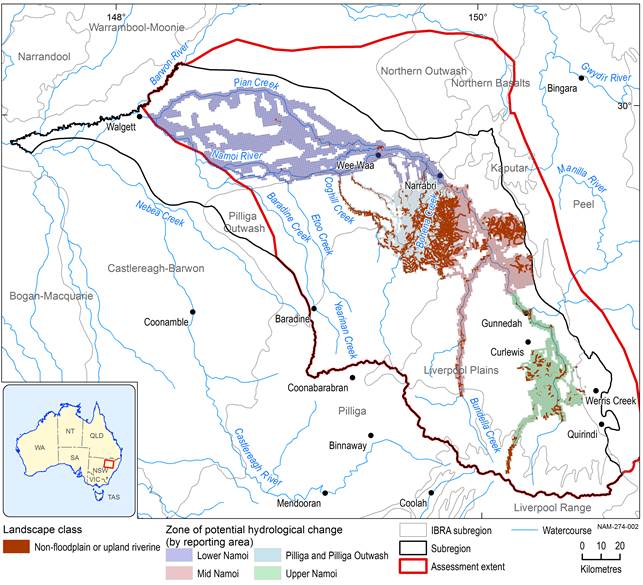
The majority (84%) of the riverine environment non-Pilliga portion of the zone of potential hydrological change in the Namoi subregion is classified as ‘Temporary upland stream’ (745.1 km or 13.5% of the zone), reflecting the intermittent or ephemeral nature of many of the stream segments (Table 18). The remainder of the stream network is classified as ‘Permanent upland stream’ (92.6 km or 1.7%), ‘Temporary upland stream GDE’ (34.7 km or 0.6%) and ‘Permanent upland stream GDE’ (14.2 km or 0.3%) (Table 18). Most of these riverine landscape classes are located in the Kaputar and Liverpool Plains Interim Biogeographic Regionalisation for Australia (IBRA) subregions (Department of Sustainability, Environment, Water, Population and Communities, Dataset 1) and form the upper reaches and tributaries of Coxs Creek, Mooki River, Maules Creek and the Namoi River (Figure 16). There are small segments of the upland riverine system classified as GDE, reflecting the gaining nature of some reaches across the zone of potential hydrological change. The hydrological connectivity within a typical upland riverine environment where the streambed is receiving water from the watertable is detailed in Figure 15.
The majority of the non-riverine landscape in the ‘Non-floodplain or upland riverine’ group in the zone of potential hydrological change is the ‘Grassy woodland GDE’ class (72.8 km2 or 1% of the zone of change; Table 18). The ‘Upland riparian forest GDE’ makes up a very small area of the zone (2.9 km2 or <0.1% of the zone) along with a small area of ‘Non-floodplain wetland’ (13.1 km2 or 0.2% of the zone) and ‘Non-floodplain wetland GDE’ landscape classes (8.1 km2 or 0.1% of the zone). These wetland classes are mostly found along the western portion of the ‘mid-Namoi’ reporting region of the zone of potential hydrological change and in the southern region of the ‘upper-Namoi’ reporting region and intersects with part of Goran Lake.
Table 18 Areas and/or lengths of the ‘Non-floodplain or upland riverine’ landscape classes within the entire assessment extent and the non-Pilliga region of the zone of potential hydrological change of the Namoi subregion
GDE = groundwater-dependent ecosystem, na = not applicable
Data: Bioregional Assessment Programme (Dataset 2)
IBRA = Interim Biogeographic Regionalisation for Australia
Data: Bioregional Assessment Programme (Dataset 2, Dataset 3); Bureau of Meteorology (Dataset 4)
Surface water flow regimes in upland riverine systems tend to be more intermittent than in lowland riverine systems for many of the streams in the Namoi region. The extent of flooding from overbank flows is reduced compared to lowland riverine systems and alluvial development tends to be confined (Figure 15).
The major stream segments of the Namoi catchment were classified into seven river ‘zones’ by Thoms (1998), each with its own set of physical characteristics. The location and extent of the zones reflect the geomorphological influences on the control of flow of water and sediment. The upland riverine landscape classes discussed here fall largely into zones associated with ‘pool’ and ‘constrained’ zones with stable channels and pool and/or run habitats (Thoms et al., 1999). The ‘armour’, ‘mobile’ and ‘meander’ zones typically have more active sediment movement from channel and bed stores and some floodplain development in the ‘meander’ zone (Thoms et al., 1999). Thoms et al. (1999) also investigated riverine health in these upland streams noting that these parts of the river systems were generally in better physical condition than those lowland parts of the Namoi river basin. Some exceptions of upland river systems with poor physical condition were the Mooki River and Coxs Creek with a lack of riparian vegetation and bank instability (Thoms et al., 1999).
Ecologically important components of the surface water regime for upland streams can be broadly summarised (Dollar, 2004) as: cease-to-flow periods, periods of low flow, freshes, and periods of high flow (including overbench and overbank flows) as illustrated in Figure 9. Further background information on the linkages between these flow components and riverine ecosystems is covered in the preceding section on lowland riverine systems (Section 2.7.3).
The riparian vegetation occurring along the upland riverine stream network is classified as ‘Grassy woodland GDE’ (72.8 km2) or ‘Upland riparian forest GDE’ (2.9 km2). The ‘Grassy woodland GDE’ landscape class is predominantly comprised of vegetation belonging to the ‘Western Slopes Grasslands’ and ‘Western Slopes Dry Sclerophyll Forests’ and ‘Brigalow Clay Plain Woodlands’ classes defined by Keith (2004). Thus, this landscape group represents a relatively diverse set of vegetation communities that occupy several different landforms with groundwater contributions from potentially different flow paths and hydrogeological units. In the eastern portion of the zone of potential hydrological change (i.e. mid-Namoi basin) the upland riverine and associated terrestrial classes (e.g. ‘Grassy woodland GDE’) are associated with basalt or permeable rock types. In these systems, groundwater is stored and transmitted through fractures, inter-granular spaces or weathered zones, and is typically discharged to the surface at contact zones between two rock types (DSITI, 2015). The ‘Upland riparian forest GDE’ class comprises the ‘Eastern Riverine Forests’ Keith class and is dominated by Casuarina cunninghamiana (river sheoak).
Credit: Bioregional Assessment Programme, Patrick Mitchell (CSIRO), January 2016
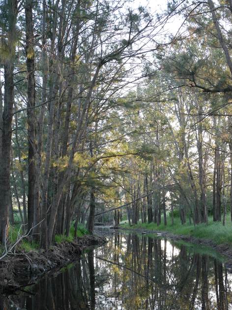
Riparian vegetation performs important functions for upland riverine ecosystems including: stabilising stream banks, filtering sediment, acting as habitat and corridors for terrestrial biota, regulating nutrient and pollutants and modifying stream microclimate (Gregory et al., 1991; Naiman and Decamps, 1997). Upland streams typical of the Namoi subregion, where the riparian vegetation is relatively intact (Figure 17), have a larger proportion of the stream that is shaded thus regulating stream conditions and limiting algal growth (Bunn, 1986). The riparian vegetation provides a large proportion of the organic carbon and other energy inputs to the surrounding catchment (Briggs and Maher, 1983; Thomas et al., 1992). The allochthonous detritus enters the stream either directly or after spending some time breaking down along the stream bank or floodplain (Reid et al., 2008). Both leaf and woody material provide important habitat structures within the stream and potential sources of carbon for some animals such as stream invertebrates and tadpoles (McKie and Cranston, 2001). These inputs of organic matter help to sustain the underlying hyporheic biota via interstitial flow through the streambed (Boulton et al., 2010).
2.7.4.1.2 Qualitative model
Upland riverine
A discussion of landscape classes for streams at the qualitative modelling workshop determined that the streams could be divided into two general groups based on their landscape classification – upland riverine and lowland riverine. The riparian vegetation and floodplain (which is only relevant for the lowland riverine group) were also included as components of the model. As described above, the upland riverine systems have intermittent flow characteristics across much of the stream network in the Namoi assessment extent. The qualitative modelling had an initial focus on populations of stream invertebrates and tadpoles inhabiting the streams in periods of flow with ecological preferences for fast- or slow-water habitats (Figure 18). These habitats are defined and enhanced by structure provided by riparian trees and other riparian vegetation, such as sedges and rushes. Riparian trees (the most common being river sheoak) provide a critical role in reducing water velocity of floods and stabilising stream banks, thereby reducing erosion and the entry of fine and suspended sediments into the stream channel (Bunn, 1986). Riparian trees are dependent on soil moisture which is replenished by overbank flows, the frequency of which was described as a specific hydrological regime (HR1). Riparian trees, sedges and rushes contribute to the structure of riparian stream habitat which benefits stream and semi-aquatic invertebrate populations, as well as mammals, reptiles, frogs and birds (Figure 18). They also contribute to stores of coarse particulate organic matter, which, when submerged, has an associated biofilm community (Figure 18). The breakdown of coarse particulate organic matter contributes to stores of fine particulate organic matter and dissolved organic matter (Figure 18). These stores of organic matter are the primary carbon (energy) source for populations of stream invertebrates and tadpoles in both slow- and fast-water habitats (Figure 18). Hyporheic biota living in subsurface sediments are sustained by the supply of particulate organic matter, dissolved organic matter and high levels of dissolved oxygen through the streambed via interstitial flow (Hose et al., 2015).
Concentrations of dissolved oxygen within the stream and streambed are influenced by flow volume (e.g. may decline during low flows and high water temperatures), and are reduced by biological oxygen demand, which depends on levels of submerged and dissolved organic matter in the stream (Reid et al., 2008) (Figure 18). Phosphorus adsorbed onto particles of suspended sediment and in runoff from cleared lands increases the growth of cyanobacteria and the likelihood of algal blooms (Figure 18). Cyanobacteria and algal photosynthesis can increase levels of dissolved oxygen during the day, and algae are an important food resource for populations of some invertebrates and tadpoles; both contribute to stores of organic matter that lead to increased levels of biological oxygen demand (Reid et al., 2008). Water temperature is regulated by the volume of streamflow, the amount of shade from riparian trees, and the proportional contribution of groundwater and water turbidity (Naiman and Decamps, 1997). High water temperatures promote cyanobacteria and reduce dissolved oxygen in stream water (Bowling and Baker, 1996). Top aquatic predators in the system include native fishes with preferences for slow- or fast-water habitats. Many species of native fishes are sensitive to the concentration of dissolved oxygen and are suppressed by high salinity and the toxic effects of cyanobacteria (Bowling and Baker, 1996).
Riparian trees in the upland riverine landscape class were described as being dependent on groundwater, such that the changes to the maximum depth of the watertable would be an important hydrologic response variable (Figure 18). River sheoaks were described as requiring periodic overbank flows for successful regeneration (Roberts and Marston, 2011). The frequency and duration of zero- and low-flow days were considered as important in maintaining slow- and fast-water habitats, riparian vegetation, and water quality (Bond et al., 2008).
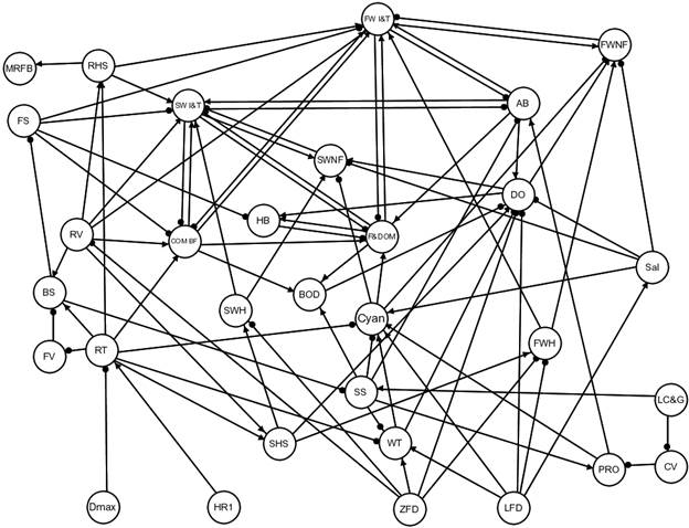
Figure 18 Signed digraph model of upland riverine landscape classes
Model variables are: algal bloom (AB), biological oxygen demand (BOD), bank stability (BS), cyanobacteria (Cyan), coarse particulate organic matter and biofilm (COM BF), catchment vegetation (CV), maximum decrease in watertable (Dmax), dissolved oxygen (DO), fine particulate and dissolved organic matter (F&DOM), fine sediments (FS), flood velocity (FV), fast-water invertebrates and tadpoles (FW I&T), fast-water habitat (FWH), fast-water native fishes (FWNF), hyporheic biota (HB), land clearing and grazing (LC&G), mammals, reptiles, frogs and birds (MRFB), phosphorous runoff (PRO), riparian habitat structure (RHS), riparian trees (RT), riparian vegetation (e.g. sedges & rushes) (RV), salinity (Sal), stream habitat structure (SHS), suspended sediment (SS), slow-water invertebrates and tadpoles (SW I&T), slow-water habitat (SWH), slow-water native fishes (SWNF), water temperature (WT), zero-flow days (ZFD), low-flow days (LFD), hydrological regime 1 (HR1).
Data: Bioregional Assessment Programme (Dataset 5)
Surface water and groundwater modelling predict significant potential impacts to hydrological regime 1 (overbank flows), low-flow days, zero-flow days, and maximum depth to groundwater level. Combinations of these impacts were considered in seven scenarios (Table 19).
Table 19 Summary of the (cumulative) impact scenarios (CISs) for upland riverine landscape classes
|
CIS |
HR1 |
LFD |
ZFD |
Dmax |
|---|---|---|---|---|
|
C1 |
– |
0 |
0 |
+ |
|
C2 |
– |
+ |
0 |
0 |
|
C3 |
– |
+ |
+ |
0 |
|
C4 |
0 |
+ |
0 |
+ |
|
C5 |
0 |
+ |
+ |
+ |
|
C6 |
– |
+ |
0 |
+ |
|
C7 |
– |
+ |
+ |
+ |
Pressure scenarios are determined by combinations of no-change (0), increase (+) or a decrease (–) in the following signed digraph variables: hydrological regime 1 (HR1, i.e. overbank flow), low-flow days (LFD), zero-flow days (ZFD), and maximum decrease in watertable (Dmax).
Data: Bioregional Assessment Programme (Dataset 5)
Qualitative analyses of the signed digraph model (Figure 18) generally indicate a negative or ambiguous response prediction for all biological variables within the upland riverine ecosystem (Table 20). Riparian trees were predicted to decrease across all of the seven cumulative impact scenarios, as were both groups of native fishes. Similarly, hyporheic fauna were predicted to decrease in all cumulative impact scenarios, while riparian vegetation (sedges and rushes) were predicted to decrease only in response to an increase in zero-flow days (i.e. C3, C5, C7).
Table 20 Predicted response of the signed digraph variables in the upland riverine landscape classes to (cumulative) changes in hydrological response variables
Qualitative model predictions that are completely determined are shown without parentheses. Predictions that are ambiguous but with a high probability (0.80 or greater) of sign determinancy are shown with parentheses. Predictions with a low probability (less than 0.80) of sign determinancy are denoted by a question mark. Zero denotes completely determined predictions of no change.
Data: Bioregional Assessment Programme (Dataset 5)
Non-floodplain wetland
The non-floodplain wetland qualitative model focused on internally draining lakes in the Namoi assessment extent, with the Lake Goran ecosystem being the primary focus, but also including Yarrie Lake (both defined as ‘Non-floodplain wetland’ landscape class). The majority of Lake Goran’s bed is frequently dry, and when lake levels are at a minimum many areas of the exposed bed are used for agriculture (Environment Australia, 2001). When the lake fills from flood events the lake water is used for irrigation. In a filled state, the lake has a number of isolated islands that provide significant roosting and nesting habitat for migratory birds. By comparison, Yarrie Lake is more permanent, smaller than Lake Goran and has no islands (Environment Australia, 2001).
The modelling exercise initially focused on the wetted area of the lake, which is increased during flood events in its catchments via local sheet flow over nearby valley slopes or channel flow in tributary streams. When the wetted area of the lake increases, it provides a surge of growth in populations of algae, macrophytes, aquatic invertebrates and fish, which are capitalised on by bird populations, including the functional groups of herbivorous, insectivorous, piscivorous and wading birds (Driver et al., 2012) (Figure 19). An increase in the wetted area of the lake favours the growth of river red gum, poplar box and lignum shrubs, with river red gum and poplar box providing critical habitat and resources for koalas, and roosting and nesting sites for populations of piscivorous, insectivorous and wading birds (Figure 19). Additionally, an increase in the wetted area provides feeding opportunities for wading birds and also contributes to roosting and nesting opportunities in predator-free areas by the isolation of islands within the lake perimeter. Lignum shrubs, and other fringing vegetation, provide habitat and resources for reptiles, frogs and terrestrial invertebrates, and populations of insectivorous birds (Figure 19).
Lignum shrubs, river red gum and poplar box depend on groundwater (Roberts and Marston, 2011). Potential impacts to this ecosystem from coal resource development includes local interception of rainfall from open-cut mines that can reduce recharge of groundwater and diminish the magnitude of sheet flow during high rainfall events (Figure 19), where this effect is localised into lowland channels adjacent to the coal mine and not tributary channels in general. Coal seam gas and open-cut coal mine development was depicted as having the potential to reduce the level of the watertable.
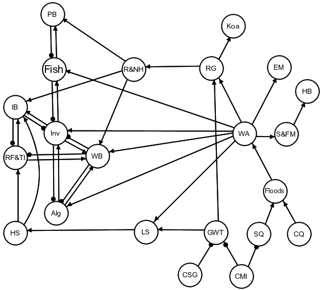
Figure 19 Signed digraph model of the 'Non-floodplain wetland' landscape class
Model variables are: algae (Alg), coal mine interception (CMI), channel flow (CQ), coal seam gas development (CSG), emergent macrophytes (EM), fish (Fish), floods (Floods), groundwater table (GWT), herbivorous birds (HB), habitat structure (HS), insectivorous birds (IB), invertebrates (Inv), koalas (Koa), lignum shrubs (LS), piscivorous birds (PB), roosting and nesting habitat (R&NH), reptiles, frogs and terrestrial invertebrates(RF&TI), river red gum (and poplar box) (RG), submerged and floating macrophytes (S&FM), sheet flow (SQ), wetted area (WA), wading birds (WB).
Data: Bioregional Assessment Programme (Dataset 5)
Surface water and groundwater modelling predict significant potential impacts to the watertable and to overland sheet flow. These potential impacts were considered in two cumulative impact scenarios that were developed for qualitative analysis of response predictions (Table 21).
Table 21 Summary of the (cumulative) impact scenarios (CISs) for the ’Non-floodplain wetland’ landscape class
|
CIS |
GWT |
SQ |
|---|---|---|
|
C1 |
– |
0 |
|
C2 |
– |
– |
Data: Bioregional Assessment Programme (Dataset 5)
Qualitative analyses of the signed digraph model (Figure 19) generally indicate a negative or ambiguous response prediction for most biological variables within the non-permanent wetland ecosystem (Table 22). Tree and shrub groups were predicted to decline in both impact scenarios, which lead to negative impacts to habitats for birds, frogs and terrestrial invertebrates. A predicted decrease in wading birds and piscivorous and insectivorous birds leads to a release, or increase, in their prey populations (i.e. fish, reptiles, frogs and terrestrial invertebrates). The potential impact of decreased sheet flow in the second cumulative impact scenario is predicted to lead to a decrease in all forms of aquatic macrophytes and herbivorous birds.
Table 22 Predicted response of the signed digraph variables in the ’Non-floodplain wetland’ landscape class to (cumulative) changes in hydrological response variables
Qualitative model predictions that are completely determined are shown without parentheses. Predictions that are ambiguous but with a high probability (0.80 or greater) of sign determinancy are shown with parentheses. Predictions with a low probability (less than 0.80) of sign determinancy are denoted by a question mark. Zero denotes completely determined predictions of no change.
Data: Bioregional Assessment Programme (Dataset 5)
2.7.4.1.3 Choice of hydrological response variables and receptor impact variables
In bioregional assessments (BAs), the potential ecological impacts of coal resource development are assessed in two future years – 2042 and 2102. These are labelled as the short- and long-assessment years, respectively. Potential ecological changes are quantified in BAs by predicting the state of a select number of receptor impact variables in the short- and long-assessment years. These predictions are made conditional on the values of certain groundwater and surface water statistics that summarise the outputs of numerical model predictions in that landscape class in an interval of time that precedes the assessment year. In all cases these predictions also allow for the possibility that changes in the future may depend on the state of the receptor impact variable in the reference year 2012, and consequently this is also quantified by conditioning on the predicted hydrological conditions in a reference interval that precedes 2012 (companion submethodology M08 (as listed in Table 1) for receptor impact modelling (Hosack et al., 2018)).
For surface water and groundwater variables in the Namoi subregion, the reference assessment interval is defined as the 30 years preceding and including 2012 (i.e. 1983 to 2012). For surface water variables in the Namoi subregion, the short-assessment interval is defined as the 30 years preceding the short-assessment year (i.e. 2013 to 2042), and the long-assessment interval is defined as the 30 years that precede the long-assessment year (i.e. 2073 to 2102). For groundwater, maximum drawdown (metres) and time to maximum drawdown are considered across the full 90-year modelling window: 2013 to 2102.
In BAs, choices about receptor impact variables must balance the project’s time and resource constraints with the objectives of the assessment and the expectations of the community (companion submethodology M10 (as listed in Table 1) for analysing impacts and risks (Henderson et al., 2018)). This choice is guided by selection criteria that acknowledge the potential for complex direct and indirect effects within perturbed ecosystems, and the need to keep the expert elicitation of receptor impact models tractable and achievable (companion submethodology M08 (as listed in Table 1) for receptor impact modelling (Hosack et al., 2018)).
For upland riverine landscape classes, the qualitative modelling workshop identified three hydrological response variables thought to: (i) be instrumental in maintaining and shaping the ecosystem and, (ii) have the potential to change due to coal resource development. All of the ecological components and processes represented in the qualitative model are potential receptor impact variables and all of these are predicted to vary as the hydrological response variables vary either individually or in combination (Table 22).
Following advice received from participants during (and after) the qualitative modelling workshop, and guided by the availability of experts for the receptor impact modelling workshop, the scope of the BA numerical modelling and the receptor impact variable selection criteria, the receptor impact models focused on the following relationships:
- The response of the upland riparian trees (RT) to changes in hydrological regime 1 (EventsR3.0) and groundwater (dmaxRef)
- The response of fast-water macroinvertebrates (FW I & T) to changes in number of zero-flow days (ZQD) and maximum length of spells with zero flow (ZME)
- The response of tadpoles (FW I & T) to changes in ZQD and ZME.
The hydrological factors identified by the participants in the qualitative modelling workshops have been interpreted as a set of hydrological response variables. The hydrological response variables are summary statistics that: (i) reflect these hydrological factors, and (ii) can be extracted from the BA’s numerical surface water and groundwater models during the reference, short- and long-assessment intervals defined previously. The hydrological factors and associated hydrological response variables for the upland riverine landscape class are summarised in Table 23. The precise definition of each receptor impact variable, typically a species or group of species represented by a qualitative model node, was determined during the receptor impact modelling workshop.
Using this interpretation of the hydrological response variables, and the receptor impact variable definitions derived during the receptor impact modelling workshop, the relationships identified in the qualitative modelling workshop were formalised into three receptor impact models (Table 24).
Table 23 Summary of the hydrological response variables used in the receptor impact models for landscape classes in the ‘Non-floodplain or upland riverine’ landscape group, together with the signed digraph variables that they correspond to
Table 24 Summary of the three receptor impact models developed for landscape classes in the ‘Non-floodplain or upland riverine’ landscape group in the Namoi subregion
Hydrological response variables are as defined in Table 23.
2.7.4.1.4 Receptor impact model
Upland riparian forest
Table 25 summarises the elicitation design matrix for the projected foliage cover of riparian trees in the upland riverine landscape classes. The first design point – design point identifier 1 – addresses the predicted variability (across the streams in the landscape class during the reference interval) in the overbank (EventsR3.0) flows that define floods with a return interval of 0.33 events per year. Note that the design point identifiers are simply index variables that identify the row of the elicitation design matrix. They are included here to maintain an auditable path between analysis and reporting.
The first design point provides for an estimate of the uncertainty in mean foliage cover across the landscape class in the reference year 2012 (Yref). The remaining design points represent hydrological scenarios that span the uncertainty in the values of the hydrological response variables in the relevant time period of hydrological history associated with the short- (2042) and long- (2102) assessment years.
Table 25 Elicitation design matrix for annual mean projected foliage cover of species group that includes: casuarina, yellow box, Blakely's red gum, Acacia salicina, Angophora floribunda, grey box in the ‘Non-floodplain or upland riverine’ landscape group in the Namoi subregion zone of potential hydrological change
Receptor impact modelling elicitation design matrix for annual mean projected foliage cover, over a 50 m x 20 m transect that extends from first bench (‘toe’) on both sides of stream in upland riparian forests. Design points for Yref in the future (short- and long-assessment periods) are calculated during the receptor impact modelling elicitation workshop using elicited values for the receptor impact variable in the reference period. All other design points (with identifiers Id) are either default values or values determined by groundwater and surface water modelling. Hydrological response variables are as described in Table 23. na = not applicable
Data: Bioregional Assessment Programme (Dataset 5)
Design point identifiers 15 through to 108 (as listed in Table 25) represent combinations of the three hydrological response variables (dmaxRef, tmaxRef, EventsR3.0), together with high and low values of Yref (see companion submethodology M08 (as listed in Table 1) for receptor impact modelling (Hosack et al., 2018)). The high and low values for Yref were calculated during the receptor impact modelling workshop following the experts’ response to the first design point, and then automatically included within the design for the elicitations at the subsequent design points.
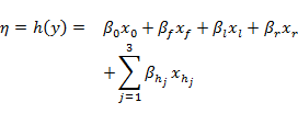
The receptor impact modelling methodology allows for a very flexible class of statistical models to be fitted to the values of the receptor impact variables elicited from the experts at each of the design points (companion submethodology M08 (as listed in Table 1) for receptor impact modelling (Hosack et al., 2018)). The model fitted to the elicited values of mean projected foliage cover for the upland riverine landscape classes is summarised in Figure 20 and Table 26. The fitted model takes the form:
|
|
where ![]() is an intercept term (a vector of ones),
is an intercept term (a vector of ones), ![]() is a binary indicator variable scored 1 for the case of an assessment in the short- or long-assessment year,
is a binary indicator variable scored 1 for the case of an assessment in the short- or long-assessment year,![]() is a binary indicator variable scored 1 for the case of an assessment in the long-assessment year,
is a binary indicator variable scored 1 for the case of an assessment in the long-assessment year, ![]() is a continuous variable that represents the value of the receptor impact variable in the reference year (Yref, set to zero for the case of an assessment in the reference year), and
is a continuous variable that represents the value of the receptor impact variable in the reference year (Yref, set to zero for the case of an assessment in the reference year), and ![]() are the (continuous or integer) values of the three hydrological response variables (dmaxRef, tmaxRef, EventsR3.0). Note that the modelling framework provides for more complex models, including quadratic value of, and in interactions between, the hydrological response variables but in this instance the simple linear model (Equation 4) was identified as the most parsimonious representation of the experts’ responses.
are the (continuous or integer) values of the three hydrological response variables (dmaxRef, tmaxRef, EventsR3.0). Note that the modelling framework provides for more complex models, including quadratic value of, and in interactions between, the hydrological response variables but in this instance the simple linear model (Equation 4) was identified as the most parsimonious representation of the experts’ responses.
The model estimation procedure adopts a Bayesian approach. The model coefficients (![]() are assumed to follow a multivariate normal distribution. The Bayesian estimation procedure quantifies how compatible different values of the parameters of this distribution are with the data (the elicited expert opinion) under the model. The (marginal) mean and 80% central credible intervals[2] of the three hydrological response variable coefficients are summarised in partial regression plots in Figure 20, whilst Table 26 summarises the same information for all seven model coefficients.
are assumed to follow a multivariate normal distribution. The Bayesian estimation procedure quantifies how compatible different values of the parameters of this distribution are with the data (the elicited expert opinion) under the model. The (marginal) mean and 80% central credible intervals[2] of the three hydrological response variable coefficients are summarised in partial regression plots in Figure 20, whilst Table 26 summarises the same information for all seven model coefficients.
The model indicates that the experts’ opinion provides strong evidence for Yref having a positive effect on average percent foliage cover. This suggests that given a set of hydrological response variable values in the future, a site with a higher foliage cover at the 2012 reference point is more likely to have a higher foliage cover in the future than a site with a lower foliage cover value at this time point. This reflects the lag in the response of foliage cover to changes in hydrological response variables that would be expected of mature trees with long life spans.
The model also indicates that the experts’ opinion provides strong evidence for dmaxRef having a negative effect on average projected foliage cover. This suggests that projected foliage cover will decrease as groundwater drawdown increases due to coal resource development. The model predicts that (holding all other hydrological response variables constant at the mid-point of their elicitation range) the mean of the average projected foliage cover will drop from just under 25% without any change in groundwater level, to about 20% if the levels decrease by 150 m relative to the reference level in 2012. There is, however, considerable uncertainty in these predictions, with an 80% chance that the foliage cover will lie somewhere between approximately 15% and 30% in the short-assessment period, and somewhere between roughly 10% and 30% in the long-assessment period, with a 6-m drop in groundwater level. In relation to dmaxRef, Yrs2tmax is also significant. The interpretation is that on average (that means for a range of drawdown from negligible to very important) long-term drawdown will have a larger effect on projected foliage cover than short-term drawdown. This is likely driven by the fact that a long-term very deep drawdown will have a more severe effect on the vegetation. Another important factor is the correlation between drawdown and time to drawdown, which will prevent some scenarios and plays a role in the marginal interpretation of the time to drawdown effect. Also note that the potential change in groundwater level relative to reference was elicited over a wide range, as the elicitations were based on preliminary groundwater modelling. Subsequent groundwater modelling identified a much lower and narrower range of drawdown as plausible than is presented in Figure 20. Predictions of projected foliage cover in the impact and risk analysis (Herr et al., 2018) use the final groundwater model results and focus only on the relationship over that narrower range.
The model indicates that the experts’ opinion provides strong evidence for EventsR3.0 having a positive effect on average projected foliage cover. The model predicts that (holding all other hydrological response variables constant at the mid-point of their elicitation range) the mean of the average projected foliage cover will increase from just under 24% without any change in overbank events frequency, to about 30% if the frequency increases to 0.8 (relative to the reference level of 0.33 in 2012).
Finally, the model also indicates some diverging influence between short-term and long-term influence. For the short-assessment period, experts believe in a relative increase of projected foliage cover, while they expect a decrease in the long-term assessment. An interpretation is that the effects of changes in hydrology are not immediate on foliage cover, and a worsening of the conditions starting today will only be observed by 2102.
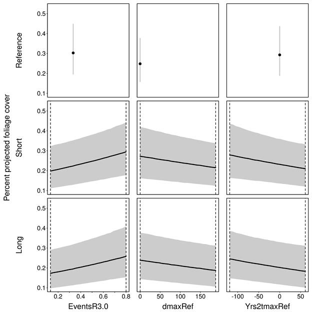
Dashed vertical lines show hydrological response variable range used in the elicitation. EventsR3.0 and dmaxRef are as described in Table 23. Yrs2tmaxRef is the difference between tmaxRef and the assessment year that is relevant for the prediction (2012, 2042 or 2102). Note that dmaxRef was elicited and is plotted over a wider range as the elicitations were based on preliminary groundwater modelling. Subsequent modelling identified a much smaller range of drawdown as plausible, and thus relevant for predicting future projected foliage cover. The numbers on the y-axis range from 0 to 1 as the receptor impact model was constructed using the proportion for the statistical modelling. They should be interpreted as a percent foliage cover ranging from 0 to 100%.
Data: Bioregional Assessment Programme (Dataset 5)
Table 26 Mean, 10th and 90th percentile of the coefficients of the receptor impact model for annual mean projected foliage cover in upland riparian forests
Future1 is the indicator variable for the short-assessment year (2042). Long1 is the indicator variable for the long-assessment year (2102). Yref quantifies the value of the receptor impact variable during the reference period. EventsR3.0 and dmaxRef are as defined in Table 23. Yrs2tmaxRef is the difference between tmaxRef and the assessment year that is relevant for the prediction (2012, 2042 or 2102).
Data: Bioregional Assessment Programme (Dataset 5)
Upland riverine
Table 27 summarises the elicitation matrix for the average number of families of aquatic macroinvertebrates from instream habitats. The first six design points – design points 1 to 7 as shown in Table 27 – address the predicted variability (across the landscape class in the reference interval) in ZQD (zero-flow days (averaged over 30 years) subsequently referred to in this section as ‘zero-flow days’) and ZME (maximum length of spells with zero flow, averaged over a 30-year period), capturing the lowest and highest predicted values together with two intermediate values. These design points provide for an estimate of the uncertainty in aquatic macroinvertebrates family abundance across the landscape class in the reference year 2012 (Yref).
Design points 10 to 22 inclusive (as listed in Table 27) represent scenarios that span the uncertainty in the predicted values of ZQD and ZME in the relevant time period of hydrological history associated with the short- (2042) and long- (2102) assessment years, combined with high and low values of Yref. Again, the high and low values for Yref were calculated during the receptor impact modelling workshop.
The fitted model for number of families of macroinvertebrates from instream habitats takes the form:
|
|
(5) |
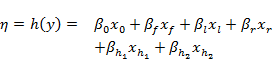
where the terms ![]() and
and ![]() are as before and
are as before and ![]() is the integer value of ZQD and
is the integer value of ZQD and ![]() is the integer value of ZME. The (marginal) mean and 80% central credible interval of the coefficient for this hydrological response variable are summarised in the partial regression plots in Figure 21, whilst Table 28 summarises the same information for all five model coefficients.
is the integer value of ZME. The (marginal) mean and 80% central credible interval of the coefficient for this hydrological response variable are summarised in the partial regression plots in Figure 21, whilst Table 28 summarises the same information for all five model coefficients.
Table 27 Elicitation design matrix for average number of families of aquatic macroinvertebrates in instream pool habitat sampled using the NSW AUSRIVAS method for pools in the ‘Non-floodplain or upland riverine’ landscape group in the Namoi subregion zone of potential hydrological change
Receptor impact modelling elicitation design matrix for the average number of families of aquatic macroinvertebrates in instream pool habitat in permanent and temporary upland streams. Design points for Yref in the future (short- and long-assessment periods) are calculated during the receptor impact modelling elicitation workshop using elicited values for the receptor impact variable in the reference period. All other design points (with identifiers Id) are either default values or values determined by groundwater and surface water modelling. ZQD and ZME are as defined in Table 23. na = not applicable
Data: Bioregional Assessment Programme (Dataset 5)
Unlike the previous model, the hydrological response variable in the macroinvertebrates model varies during the reference interval and the future interval. The model indicates that the experts’ elicited information strongly supports the hypothesis that an increase in ZQD and/or ZME will have a negative effect on the number of families of macroinvertebrates despite the experts being quite uncertain about its average value. The model suggests that it can vary substantially across the landscape class from less than 5 to almost 20 under conditions of constant flow (ZQD = zero), holding all other covariates at their mid-values. As the number of zero-flow days increases, however, experts were of the opinion that the number of families would drop quite dramatically with values <0.5 falling within the 80% credible interval under very intermittent flow conditions (ZQD >300 days) (Figure 21).
There was very little evidence in the elicited data to suggest that this effect would be substantially different in the future assessment years. Again, this is indicated by the almost identical partial regression plots in the reference, short- and long-assessment years (Figure 21), and the relatively large negative 10th and positive 90th percentiles for the long and future coefficients in Table 28. The model does, however, suggest that the experts’ uncertainty increased for predictions in the future assessment years relative to the reference year.
Another notable difference between this model and the previous model is the estimated values for the Yref coefficient. In the projected foliage cover model, there was strong evidence within the experts’ elicited values that the average percent foliage cover in the reference year had a positive influence on the values in the future assessment years ![]() ). The best-fitting model in this case, however, is unable to eliminate the possibility that the average number of families of macroinvertebrates in the reference years has no influence on its number in the future years. This is indicated by the fact the model automatically dropped this variable from the model. This suggestion is consistent with the hypothesis that there is likely to be very little lag in the response of this short-lived group to changes in the hydrological response variables.
). The best-fitting model in this case, however, is unable to eliminate the possibility that the average number of families of macroinvertebrates in the reference years has no influence on its number in the future years. This is indicated by the fact the model automatically dropped this variable from the model. This suggestion is consistent with the hypothesis that there is likely to be very little lag in the response of this short-lived group to changes in the hydrological response variables.
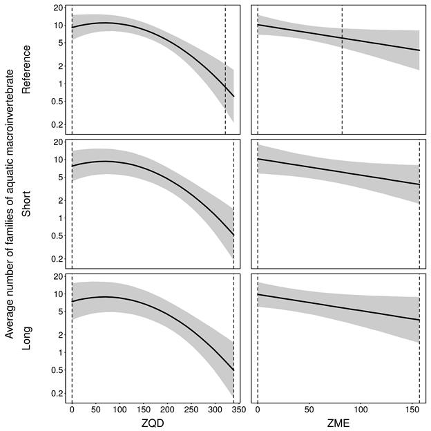
Dashed vertical lines show hydrological response variable range used in the elicitation. ZQD and ZME are as defined in Table 23.
Data: Bioregional Assessment Programme (Dataset 5)
Table 28 Mean, 10th and 90th percentile of the coefficients of the receptor impact model for the average number of families of aquatic macroinvertebrates in instream pool habitat in upland riverine landscape classes
|
|
Mean |
q10 |
q90 |
|---|---|---|---|
|
(Intercept) |
2.47 |
2.06 |
2.88 |
|
future1 |
0.0762 |
–0.41 |
0.562 |
|
long1 |
–0.0466 |
–0.614 |
0.521 |
|
ZQD |
0.0054 |
–0.000288 |
0.0111 |
|
ZME |
–0.00641 |
–0.0128 |
–3.85e-05 |
|
I(ZQD^2) |
–3.95e-05 |
–6.04e-05 |
–1.86e-05 |
Future1 is the indicator variable for the short-assessment year (2042). Long1 is the indicator variable for the long-assessment year (2102). ZQD and ZME are as defined in Table 23. I(ZQD^2) quantifies the quadratic effect of ZQD.
Data: Bioregional Assessment Programme (Dataset 5)
Table 29 summarises the elicitation matrix for the probability of presence of tadpoles from the Limnodynastes genus (dumerilii, salmini, interioris and terraereginae). The first six design points – design points 1 to 7 as shown in Table 29 – address the predicted variability (across the landscape class in the reference interval) in ZQD and ZME, capturing the lowest and highest predicted values together with two intermediate values. These design points provide for an estimate of the uncertainty in probability of presence of tadpoles across the landscape class in the reference year 2012 (Yref).
Table 29 Elicitation design matrix for probability of presence of tadpoles from Limnodynastes genus (dumerilii, salmini, interioris and terraereginae) in the ‘Non-floodplain or upland riverine’ landscape group in the Namoi subregion zone of potential hydrological change
Receptor impact modelling elicitation design matrix for the probability of presence of tadpoles in pools and riffles in permanent and temporary upland streams. Design points for Yref in the future (short- and long-assessment periods) are calculated during the receptor impact modelling elicitation workshop using elicited values for the receptor impact variable in the reference period. All other design points (with identifiers Id) are either default values or values determined by groundwater and surface water modelling. ZQD and ZME are as defined in Table 23. na = not applicable
Data: Bioregional Assessment Programme (Dataset 5)
Design points 10 to 22 inclusive (as listed in Table 29) represent scenarios that span the uncertainty in the predicted values of ZQD and ZME in the relevant time period of hydrological history associated with the short- (2042) and long- (2102) assessment years, combined with high and low values of Yref. Again, the high and low values for Yref were calculated during the receptor impact modelling workshop.
The fitted model for probability of the presence of tadpoles takes the form:
|
|
(6) |
where the terms ![]() and
and ![]() are as before and
are as before and ![]() is the integer value of ZQD and
is the integer value of ZQD and ![]() is the integer value of ZME. The (marginal) mean and 80% central credible interval of the coefficient for this hydrological response variable are summarised in the partial regression plots in Figure 22, whilst Table 30 summarises the same information for all six model coefficients.
is the integer value of ZME. The (marginal) mean and 80% central credible interval of the coefficient for this hydrological response variable are summarised in the partial regression plots in Figure 22, whilst Table 30 summarises the same information for all six model coefficients.
Like the previous model, the hydrological response variable in the tadpole model varies during the reference interval and the future interval. The model indicates that the experts’ elicited information strongly supports the hypothesis that an increase in ZQD and/or ZME will have a negative effect on probability of the presence of tadpoles. The model suggests that the probability of tadpoles is fairly high with low uncertainty across the landscape classes with a value of almost 1 under conditions of constant flow (ZQD = zero), holding all other covariates at their mid-values. As the number of zero-flow days increases, however, experts were of the opinion that the probability of presence would drop quite dramatically with values <0.1 falling within the 80% credible interval under very intermittent flow conditions (ZQD >300 days) (Figure 22).
There was very little evidence in the elicited data to suggest that this effect would be substantially different in the future assessment years. Again, this is indicated by the almost identical partial regression plots in the reference, short- and long-assessment years (Figure 22), and the relatively large negative 10th and positive 90th percentiles for the long and future coefficients in Table 30. The model does, however, suggest that the experts’ uncertainty increased for predictions in the future assessment years relative to the reference year.
Like the previous model, the best-fitting model in this case is unable to eliminate the possibility that the probability of the presence in the reference years has no influence on the probability of the presence in the future years. This is indicated by the fact the model automatically dropped this variable from the model. This suggestion is consistent with the hypothesis that there is likely to be very little lag in the response of this short-lived group to changes in the hydrological response variables.
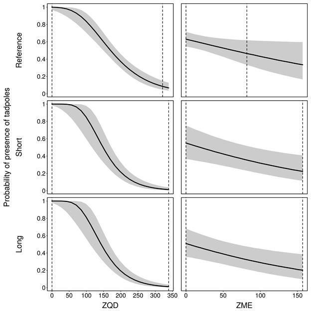
Dashed vertical lines show hydrological response variable range used in the elicitation. ZQD and ZME are as defined in Table 23.
Data: Bioregional Assessment Programme (Dataset 5)
Table 30 Mean, 10th and 90th percentile of the coefficients of the receptor impact model for the probability of the presence of tadpoles in pools and riffles in upland riverine landscape classes
|
|
Mean |
q10 |
q90 |
|---|---|---|---|
|
(Intercept) |
0.942 |
0.36 |
1.52 |
|
future1 |
–0.169 |
–0.734 |
0.396 |
|
long1 |
–0.113 |
–0.762 |
0.535 |
|
ZQD |
–0.00589 |
–0.0093 |
–0.00248 |
|
ZME |
0.0243 |
0.00842 |
0.0401 |
|
ZQD:ZME |
–0.000186 |
–0.000271 |
–0.000102 |
Future1 is the indicator variable for the short-assessment year (2042). Long1 is the indicator variable for the long-assessment year (2102). ZQD and ZME are as defined in Table 23. ZQD:ZME quantifies the effect of the interaction between ZQD and ZME.
Data: Bioregional Assessment Programme (Dataset 5)
