In BA, receptor impact models for ecological water-dependent assets are conditioned upon, and therefore depend on, landscape classes. A landscape class is defined as an ecosystem with characteristics that are expected to respond similarly to changes in groundwater and/or surface water due to coal resource development. Each bioregion or subregion has multiple landscape classes grouped into landscape groups.
The workflow for ecological receptor impact modelling is outlined in Figure 3. Input from independent external ecology experts contributes to the workflow at three separate stages (2, 3 and 5 in Figure 3), along with output from hydrological modelling (companion product 2.6.1 (Aryal et al., 2018) and companion product 2.6.2 (Janardhanan et al., 2018) for the Namoi subregion) and the expertise of the hydrology modellers. External experts, hydrologists and risk analysts contribute to the selection of hydrological response variables that are ecologically meaningful and also accessible to hydrological modelling. The expert elicitation data are available as a downloadable dataset from data.gov.au.
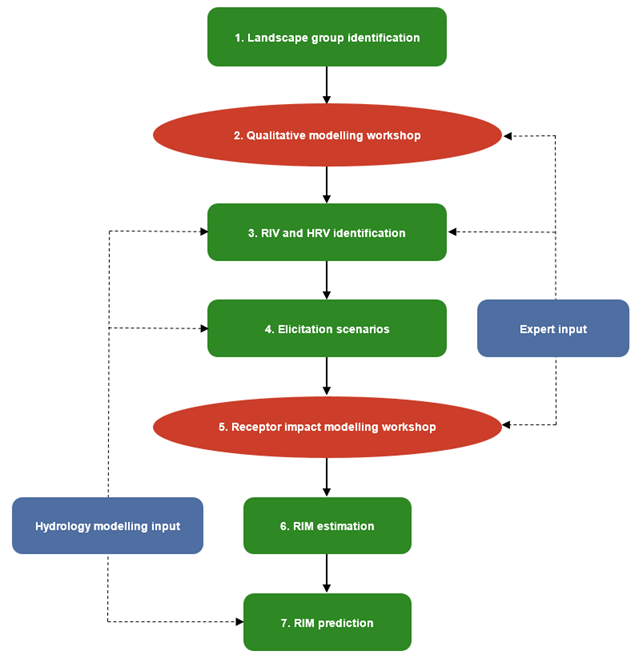
In this figure the green boxes represent specific stages undertaken by the Assessment team in the overall receptor impact modelling process, the red boxes are the two external workshops and the blue boxes are external expert or modelling inputs.
HRV = hydrological response variable, RIM = receptor impact model, RIV = receptor impact variable
The workflow shown in Figure 3 leads to the construction of a receptor impact model that predicts the response of a receptor impact variable to changes in hydrological response variables. The receptor impact models propagate the uncertainty in: (i) the effect of coal resource development on the hydrological response variables under the baseline and CRDP; and, (ii) the uncertainty in the receptor impact variable response to these hydrological changes across a landscape class.
2.7.1.2.1 Identification of landscape classes that are potentially impacted
BAs identify landscape classes (Stage 1 in Figure 3) that could be impacted by coal resource development as those landscape classes that lie wholly or partially within the zone of potential hydrological change. The zone of potential hydrological change is defined as the union of the groundwater and surface water zones of potential hydrological change. The groundwater zone of potential hydrological change is defined as the area with a greater than 5% chance of exceeding 0.2 m of drawdown in the relevant aquifers (see companion submethodology M10 (as listed in Table 1) for analysing impacts and risks (Henderson et al., 2018)). In the BA for the Namoi subregion, the relevant aquifer is the regional watertable.
The surface water zone of potential hydrological change is defined in a similar manner. The area contains those river reaches where a change in at least one of nine surface water hydrological response variables exceeds its specified threshold. For the four flux-based hydrological response variables – annual flow (AF), daily flow rate at the 99th percentile (P99), interquartile range (IQR) and daily flow rate at the 1st percentile (P01) – the threshold is a 5% chance of a 1% change in the variable, with an additional threshold specified for P01 (see Table 4 in companion product 3-4 for the Namoi subregion (Herr et al., 2018a)). That is, if 5% or more of model runs show a maximum change in results under CRDP of 1% relative to baseline. For four of the frequency-based hydrological response variables – high-flow days (FD), low-flow days (LFD), length of low-flow spell (LLFS) and zero-flow days (ZFD) – the threshold is a 5% chance of a change of three days per year. For the final frequency-based hydrological response variable (low-flow spells, LFS), the threshold is a 5% chance that the maximum difference in the number of low flow spells between the baseline and CRDP futures is at least two spells per year (companion submethodology M06 (as listed in Table 1) for surface water modelling (Viney, 2016)).
It is important to recognise that the zone of potential hydrological change identifies those parts of the landscape where there is at least a 5% chance of a small (as defined by hydrological thresholds used) hydrological change attributable to coal resource development. The zone serves only to identify those landscape classes that should be taken to the next step of the receptor impact methodology from those landscape classes that should not, on the grounds that the latter are predicted to experience negligible (or insignificant) exposure to hydrological change due to coal resource development.
2.7.1.2.2 Qualitative mathematical modelling of landscape classes
BAs use qualitative mathematical models to describe landscape class ecosystems, and to predict (qualitatively) how coal resource development will directly and indirectly affect these ecosystems. Qualitative mathematical models were constructed in dedicated workshops, attended by experts familiar with these landscapes and/or the Namoi subregion (Table 3; Stage 2 in Figure 3). In the workshop, ecological and hydrological experts were asked to describe how the key species and/or functional groups within the landscape class ecosystem interact with each other, and to identify the principal physical processes that mediate or otherwise influence these interactions. During this process the experts were also asked to identify how key hydrological processes support the ecological components and processes of the landscape class. The experts’ responses were formally translated into qualitative mathematical models which enable the BA team to identify critical relationships and variables that will become the focus of the quantitative receptor impact models.
Table 3 List of organisations with experts participating in the Namoi subregion qualitative mathematical modelling (QMM) and receptor impact modelling (RIM) workshops
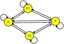
Qualitative modelling proceeds from the construction and analysis of sign-directed graphs, or signed digraphs, which are depictions of the variables and interactions of a system. These digraphs are only concerned with the sign (+, –, 0) of the direct effects that link variables. For instance, the signed digraph in Figure 4 depicts a straight-chain system with a basal resource (R), consumer (C) and predator (P). There are two predator-prey relationships, where the predator receives a positive direct effect (i.e. nutrition, shown as a link ending in an arrow (![]() )), and the prey receives a negative direct effect (i.e. mortality, shown as a link ending in a filled circle (
)), and the prey receives a negative direct effect (i.e. mortality, shown as a link ending in a filled circle (![]() )). The signed digraph also depicts self-effects, such as density-dependent growth, as links that start and end in the same variable. In the example in Figure 4 these self-effects are negative.
)). The signed digraph also depicts self-effects, such as density-dependent growth, as links that start and end in the same variable. In the example in Figure 4 these self-effects are negative.
The structure of a signed digraph provides a basis to predict the stability of the system that it portrays, and also allows the analyst to predict the direction of change of all the model’s variables (i.e. increase, decrease, no change) following a sustained change to one (or more) of its variables. The signed digraph in Figure 4, for example, is stable because: (i) it only has negative feedback cycles, (ii) the paths leading from the predators to their prey and back to the predator are negative feedback cycles of length two, and (iii) there are no positive (destabilising) cycles in the system. This model therefore predicts that if this system were to experience a sudden disturbance it would be expected to return relatively quickly to its previous state or equilibrium.
The predicted direction of change of the variables within a signed digraph to a sustained change in one or more of its variables is determined by the balance of positive and negative effects through all paths in the model that are perturbed. Consider, for example, a pressure to the system depicted in Figure 4 that somehow supplements the food available to the predator P causing it to increase its reproductive capacity. The predicted response of C is determined by the sign of the link leading from P to C, which is negative (denoted as P ![]() C). The predicted response of R will be positive because there are two negative links in the path from P to R (P
C). The predicted response of R will be positive because there are two negative links in the path from P to R (P ![]() C
C ![]() R), and their sign product is positive (i.e. − x − = +).
R), and their sign product is positive (i.e. − x − = +).
In the system depicted in Figure 4, the response of the model variables (P, C, R) to a sustained pressure will always be unambiguous – the predictions are said to be completely sign determined. This occurs in this model because there are no multiple pathways between variables with opposite signs.
By way of contrast, the signed digraph depicted in Figure 5 is more complex because it includes an additional consumer and a predator that feeds on more than one trophic level. This added complexity creates multiple pathways with opposite signs between P and R.
Here the predicted response of R due to an increase in P will be ambiguous, because there are now three paths leading from P to R, two positive (P ![]() C1
C1 ![]() R, P
R, P ![]() C2
C2 ![]() R) and one negative (P
R) and one negative (P ![]() R). The abundance of the resource may therefore increase or decrease. This ambiguity can be approached in two ways. One is to apply knowledge of the relative strength of the links connecting P to R. If P was only a minor consumer of R then the R would be predicted to increase. Alternatively, if R was the main prey of P, and C1 and C2 amounted to only a minor portion of P’s diet, then R would be predicted to decrease in abundance.
R). The abundance of the resource may therefore increase or decrease. This ambiguity can be approached in two ways. One is to apply knowledge of the relative strength of the links connecting P to R. If P was only a minor consumer of R then the R would be predicted to increase. Alternatively, if R was the main prey of P, and C1 and C2 amounted to only a minor portion of P’s diet, then R would be predicted to decrease in abundance.
In many cases, however, there is insufficient knowledge of the strength of the links involved in a response prediction. In these instances, Dambacher et al. (2003) and Hosack et al. (2008) described a statistical approach that estimates the probability of sign determinacy for each response prediction. In the Figure 5 example, with two positively signed paths and one negatively signed path, there is a net of one positive path (i.e. it is considered that a negatively signed path cancels a positively signed path) out of a total of three paths. According to this approach, in the system depicted in Figure 5, R is predicted to increase 77% of the time because of the ratio of the net to the total number of paths.
The ratio of the net to the total number of paths in a response prediction has been determined to be a robust means of assigning probability of sign determinacy to response predictions. These probabilities of sign determinacy can then be used to assess cumulative impacts that result from a perturbation to the system.
2.7.1.2.3 Choice of hydrological response variables and receptor impact variables
In BAs, qualitative mathematical models are used to represent how ecosystems will respond qualitatively (increase, decrease, no change) to changes in the hydrological variables that support them. The models also provide a basis for identifying receptor impact variables and hydrological response variables that are the subject of the quantitative receptor impact models (Stage 3 in Figure 3).
The qualitative mathematical models identify a suite of ecologically important water requirements that support the landscape class ecosystem. These variables are sometimes expressed as hydrological regimes, for example an overbank flow regime premised on an average recurrence interval of once every three years. The hydrological components in these models are linked to the hazard analysis (companion submethodology M11 (as listed in Table 1) for hazard analysis (Ford et al., 2016)) and provide the mechanism via which the coal resource development can adversely affect groundwater and surface water dependent ecosystems.
Hydrological response variables are derived from the numerical surface water and groundwater model results to represent these ecologically important water requirements. The surface water hydrological response variables in the receptor impact models are defined in terms of mean annual values for two 30-year periods: 2013 to 2042 and 2073 to 2102 (e.g. mean number of zero-flow days per year between 2013 and 2042). The hydrological response variables are generalised for the assessment extent and thus serve as indicators of change in ecologically important flows, rather than accurate characterisation of flow regimes at local scales. They differ from the hydrological response variables defined in companion product 2.6.1 for surface water modelling in the Namoi subregion (Aryal et al., 2018), which represent the maximum difference between the CRDP and baseline simulations over the 90-year simulation period (e.g. the maximum difference in zero-flow days per year between 2013 and 2102).
Receptor impact variables are selected according to the following criteria:
- Is it directly affected by changes in hydrology? These variables typically have a lower trophic level.
- Is it representative of the broader landscape class? Variables (or nodes) within the qualitative model that other components of that ecosystem or landscape class depend on will speak more broadly to potential impacts.
- Is it something that expertise available can provide opinion on? There is a need to be pragmatic and make a choice of receptor impact variable that plays to the strengths of the experts available.
- Is it something that is potentially measurable? This may be important for validation of the impact and risk analysis.
- Will the choices of receptor impact variable for a landscape class resonate with the community? This speaks to the communication value of the receptor impact variable.
Receptor impact variables are chosen as indicators about the response of a landscape class. Changes in the receptor impact variables (e.g. foliage cover, taxa richness) imply changes to the ecology of the landscape class. A decrease in projected cover of woody riparian vegetation implies a reduction in the abundance and/or health of trees along river banks. A receptor impact variable may coincide with an ecological asset. For example, the abundance of a species listed under the Commonwealth’s Environment Protection and Biodiversity Conservation Act 1999 (EPBC Act), whose modelled ‘Habitat (potential species distribution)’ is an asset, might be selected as an indicator of overall ecosystem condition if experts thought its abundance were highly sensitive to hydrological change. Alternatively, a receptor impact variable that is not an asset, but which is highly sensitive to hydrological change, may be a useful indicator of the overall response of a given asset or landscape class.
The goal of the receptor impact modelling workshop (Stage 5 in Figure 3) is to predict how a given receptor impact variable will respond at future time points to changes in the values of hydrological response variables, whilst acknowledging that this response may be influenced by the status and condition of the receptor impact variable in the reference year (2012). Response variables to represent changes in water quality that might be expected to accompany changes in the relative contributions of surface runoff and groundwater to streamflow are not included in the models or the elicitations.
The elicitation generates subjective probability distributions for the expected value of the receptor impact variable under a set of hydrological scenarios that represent possible combinations of changes to hydrological response variables. These scenarios are the elicitation equivalent of a sampling design for an experiment where the aim is to maximise the information gain and minimise the cost. The same design principles therefore apply (Stage 4 in Figure 3).
It is essential to have an efficient design to collect the expert information, given the large number of receptor impact models, landscape classes, and bioregions and subregions to address within the operational constraints of the programme. The design must also respect, as much as possible, the predicted hydrological regimes as summarised by hydrological modelling outputs. Without this information, design points may present hydrological scenarios that are unrealistically beyond bounds suggested by the landscape class definition. Alternatively, insufficiently wide bounds on hydrological regimes lead to an over-extrapolation problem when receptor impact model predictions are made conditional on hydrological simulations at the risk-estimation stage (Stage 6 in Figure 3). The design must further respect the feasibility of the design space, which may be constrained by mathematical relationships between related hydrological response variables. The design must accommodate the requirement to predict to past and future assessment years. The design must also allow for the estimation of potentially important interactions and nonlinear impacts of hydrological response variables on the receptor impact variable.
2.7.1.2.4 Construction and estimation of receptor impact models
BAs address the question ‘How might selected receptor impact variables change under various scenarios of change for the hydrological response variables?’ through formal elicitation of expert opinion. This is a difficult question to tackle and presents a challenging elicitation task. BAs implement a number of processes that are designed to help meet this challenge: (i) persons invited to the receptor impact modelling workshops are selected based on the relevance of their domain expertise; (ii) all experts are provided with pre-workshop documents that outline the approach, the expectations on the group and the landscape classes and descriptions, and subsequently the finalised qualitative models; and (iii) experts are given some training on subjective probability, common heuristics and biases, together with a practice elicitation.
The elicitation proper follows a five-step procedure (described in detail in companion submethodology M08 (as listed in Table 1) for receptor impact modelling (Hosack et al., 2018)) that initially elicits fractiles, fits and plots a probability density function to these fractiles, and then checks with the experts if fractiles predicted by the fitted density are sufficiently close to their elicited values. This process is re-iterated until the experts confirm that the elicited and fitted fractiles, and the fitted lower (10th) and upper (90th) fractiles, provide an adequate summary of their opinions for the elicitation scenario concerned.
The experts’ responses to the elicitations are treated as data inputs into a Bayesian generalised linear model (Stage 6 in Figure 3; see submethodology M08 (as listed in Table 1) for receptor impact modelling (Hosack et al., 2018)). The model estimation procedure allows for a wide variety of possible model structures that can accommodate quadratic responses of receptor impact variables to changes in hydrological response variables, and interactive (synergistic or antagonist) effects between hydrological response variables. The procedure uses a common model selection criterion (the Bayesian Information Criterion) to select the model that most parsimoniously fits the experts’ response to the elicitation scenarios.
2.7.1.2.5 Receptor impact model prediction
This stage (Stage 7 in Figure 3) applies the receptor impact model methodology to predict the response of the receptor impact variables. The general framework allows for the receptor impact model to be applied either at single or multiple receptor locations (assessment units). The receptor impact model can therefore be applied at multiple receptor locations that are representative of a landscape class within a bioregion or subregion. The primary endpoint considered, however, is predicting receptor impact variable response to the BA future across an entire landscape class, which is accomplished by including all locations (assessment units) that represent the hydrological characteristics of the landscape class. The uncertainty from the hydrology modelling is propagated through the receptor impact model at each location to give the predicted distribution of the receptor impact variable at different time points for the two futures considered by BA (baseline and CRDP). The uncertainties are then aggregated to give the response across the entire landscape class. Companion submethodology M09 (as listed in Table 1; Peeters et al., 2016) provides further details on how uncertainty is propagated through the hydrological models. Integrating across these receptors produces the overall predicted response of the receptor impact variable for the landscape class given the choice of the BA future. These landscape class results are summarised in product 3-4 (impacts and risks) for the Namoi subregion (Herr et al., 2018a). The results do not replace the need for detailed site or project specific studies, nor should they be used to pre-empt the results of detailed studies that may be required under state and Commonwealth legislation. Detailed site studies may give differing results due to the scale of modelling used.
2.7.1.2.6 Receptor impact modelling assumptions and implications
The receptor impact modelling methodology (companion submethodology M08 (as listed in Table 1; Hosack et al., 2018)) and its implementation was affected by design choices that have been made within BA. Some of these broader choices are described in companion submethodology M10 (as listed in Table 1) for analysing impacts and risks (Henderson et al., 2018). Table 4 summarises some of the assumptions made for the receptor impact modelling, the implications of those assumptions for the results, and how those implications are acknowledged through the BA products.
Table 4 Summary of the receptor impact modelling assumptions, their potential implications, and their acknowledgement through BA products
|
Assumptions of receptor impact modelling |
Implications |
Acknowledgement |
|---|---|---|
|
Discretisation of continuous landscape surface |
Provided a defined spatial scope for experts to address. Connections between landscape classes broken. Changes in one landscape class may have implications for adjacent landscape classes |
Identify potential connections between landscape classes where possible in the impact and risk product. Some qualitative mathematical models do include links to nearby landscape classes |
|
Data underpinning landscape classes is sufficient and correct |
Landscape class definition required data input from pre-existing data sources. Prioritisation for qualitative mathematical models and receptor impact models may be affected. Minimal effect on model development for receptor impact models |
Acknowledge issues with data in the impact and risk product (also done in the conceptual modelling product). In companion product 3-4 for the Namoi subregion (Herr et al., 2018a) acknowledge that mapped results reflect the mapped inputs |
|
Areas of landscape classes are constant over modelling period |
Provides a defined spatial scope for expert assessment of change. BA is about identifying existing areas that are at risk from coal resource development as opposed to predicting the changes in areal extent or transition to different landscape classes. Some potential for changes in the area of the landscape class to affect its sensitivity to hydrological change but would need to be assessed on an asset-by-asset basis |
Acknowledge in Methods |
|
Other developments and users of water (e.g. agriculture) are constant over time |
Provided a defined context for experts to consider. BA is about identifying existing areas that are at risk from coal resource development as opposed to predicting the changes due to other developments or the relative attribution |
Acknowledge in Methods |
|
Landscape characteristics other than hydrological variables are not represented in quantitative receptor impact models |
Limits hydrological response variables used in receptor impact models to those that may be derived from hydrological models developed by BA. The absence of water quality variables is a noted limitation. Loss of within-landscape class predictive performance from the receptor impact models |
Identify as knowledge gap when the hydrological response variables used in the model represent a subset of the key dependencies. Acknowledge importance of local (vs regional) analyses where the concern is over particular parts of a landscape class |
|
Experts available adequately represent the state of knowledge for relevant landscape classes |
Experts provided domain expertise and experience that informed both model structure and also provided quantifiable predictions of receptor impact variable response to novel hydrological scenarios. Expert availability affected the quality/utility of the qualitative mathematical model; identification of receptor impact variables that reflect expertise of those in the room |
Acknowledge that the receptor impact variable is an ‘indicator’ of the potential ecosystem response. Identify as knowledge gap where part of the landscape class is not represented |
|
The simplification of complex systems is appropriate for the task |
Provided formal approach to model identification and selection of candidate receptor impact variables. Not all components and relationships are represented by receptor impact models |
Acknowledge that one or two receptor impact variables can underestimate complex ecosystem function. Make assumptions clear. High-level interpretation of results. Emphasise importance of interpreting the hydrological change |
|
A common set of modelled hydrological response variables is appropriate across different landscape classes |
Limits hydrological response variables used in receptor impact models to those that may be derived from hydrological models developed by BA. Enables some simplification of complex systems. Loss of local specificity in predictions of receptor impact variables |
The need for local-scale information is identified (in multiple places) |
|
Receptor impact variables are good indicators of ecosystem response |
The qualitative models informed the selection of receptor impact variables within the additional constraints imposed by expert availability given project timelines. Focus of the quantified relationships within the landscape class |
The need for local-scale information is identified (in multiple places) |
|
Extrapolation of predictions beyond elicitation scenarios |
The ranges of hydrological scenarios to be considered at the expert elicitation sessions were informed by preliminary hydrological modelling output and hydrological expert advice within BA. However, final model results sometimes extended beyond this preliminary range due to necessary changes in underlying hydrological modelling assumptions and assimilation of data. Extrapolation beyond the range of hydrological response variables considered by the expert elicitation increases uncertainty in receptor impact variable predictions |
Identify as a limitation for the appropriate landscape class in the impact and risk product where this occurs |
|
Qualitative mathematical models focus on impacts of long-term sustained hydrological changes (press perturbations) to ecosystems. The quantitative receptor impact models can and do account for pulse perturbations and associated responses, where experts were free to include direct and indirect effects as well as pulse and press perturbations within their assessments |
Qualitative models may not accurately represent impacts of shorter-term hydrological changes (pulse perturbations) on ecosystems and landscape classes |
Describe rationale for the focus on press perturbations in companion submethodology M08 (as listed in Table 1) for receptor impact modelling (Hosack et al., 2018). Note that many potential pulse perturbations are caused by accidents and managed by site-based processes. Identify as a limitation / knowledge gap. Note that quantitative receptor impact models do account for pulse perturbations |
BA = bioregional assessment
