The allocation of receptors was undertaken as a staged process. The preliminary distribution of model nodes was assigned using the Bureau of Meteorology’s Geofabric (Dataset 1). The Geofabric is a specialised GIS consisting of nationally consistent spatial data that identifies important water features in the landscape, and the connectivity between these water bodies. Detailed descriptions of the Geofabric can be found in the Geofabric product guide (Bureau of Meteorology, 2012). The Geofabric identifies approximately 7800 surface water river basins in the Namoi subregion. River basins are delineated in a hierarchical fashion and each has a unique code (based on the Pfafstetter Coding system, developed by Otto Pfafstetter (1989); a methodology for assigning unique river basin IDs based on the topology of the land surface – sometimes referred to herewith using a shortened form of ‘Pfaf’).
Table 4 Preliminary classification of landscape classes of the Namoi subregion based on surface water characteristics
Example only; do not use for analysis.
Surface water modelling in the Namoi will be initialised using a rainfall-runoff model with a 0.5 degree resolution (~2500 ha grid). This delineates the minimum resolution of the hydrological modelling within the Geofabric surface water river basin hierarchy. In the Namoi subregion, ‘Pfafstetter 8’ river basins were identified for initialisation of the distribution of receptors as most river basins at this scale were larger than 2500 ha. By intersecting the existing Geofabric node network with the 9-second DEM (i.e. a digital elevation model with approximately 300 m grid cell resolution), the node at the lowest point in each ‘Pfafstetter 8’ river basin was selected as the receptor for that surface water river basin. This resulted in a distribution of receptors across the surface water network shown in Figure 10. The same procedure was run for ‘Pfafstetter 9’ river basins and for ‘Pfafstetter 10’ river basins. The resultant distribution of receptors is shown in Figure 11.
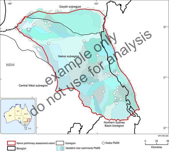
Figure 10 Preliminary distribution of surface water receptors for the Namoi subregion
Receptors represent the lowest Geofabric node, identified using a 9-second digital elevation model (DEM), in each of ‘Pfafstetter 8 river basins.
Data: example data derived from Bureau of Meteorology (Dataset 1)
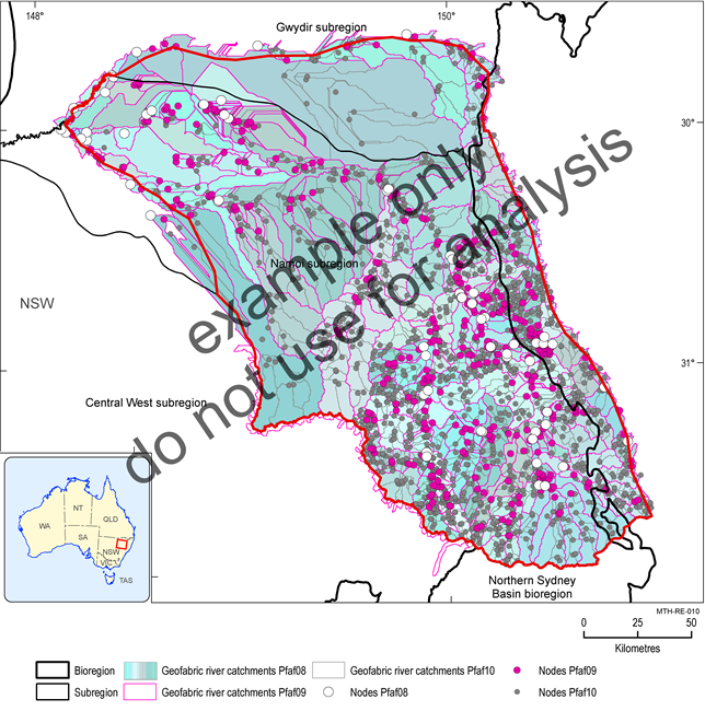
Receptors were chosen by selecting the lowest nodes in each of ‘Pfafstetter 8,9 and 10’ river basins within the Geofabric.
Data: example data derived from Bureau of Meteorology (Dataset 1)
Two important questions need to be answered at this point in the process:
- What is a representative distribution of receptors? In particular, how representative are the receptors of the assets and the potential impacts upon them?
- How to interpolate responses from the model emulators to individual receptors associated with assets?
A number of approaches could be used to assess the representativeness of the surface water receptor distribution. Ultimately both questions need to be decided by the Assessment team working in close collaboration – particularly the hydrologists, the ecologists and the risk experts. In the example, representativeness was assessed by examining the number of landscape classes within 1, 2.5, 5, 10 and 20 km of the receptor node. In the ‘Pfafstetter 8’ river basins a radius of greater than 20 km was required to intersect with the 18 landscape classes in the BA; in the ‘Pfafstetter 10’ river basins, this radius was reduced to 5 km (Table 5). In this example a core principle was to minimise the internal heterogeneity. Alternative indicators of representativeness are clearly possible (e.g. the density of receptors per landscape class or some other areal unit. Whatever indicator of representativeness is used, the choice of receptor placement and density needs to support an objective assessment of potential impact. An asset that is fairly homogeneous may be adequately assessed by fewer receptors than one that is more diverse.
A complete distribution of receptors was achieved by placing a receptor on each polygon at the nearest point of each element in each asset class (Figure 12). For pragmatic purposes, in this example, a point on the edge closest to the node was selected. However, the Assessment team could define the rules related to the placement of the receptor that are relevant to the landscape class (e.g. centroids).
The outcome of this step is that there is a receptor associated with every element in each landscape class. While complete, this may not be an efficient distribution as there may be many thousands of receptors that are redundant; similarly, the distribution of receptors in large assets should be checked for representativeness. Existing approaches, such as that outlined by Stevens and Olsen (2004), might be used to help decide on the final, refined distribution of receptors for inclusion in the receptor register.
Table 5 Number of landscape elements within each landscape class in relation to nodes from three Pfafstetter classifications
Values within each row represent the number of elements within set distances of the receptors. Note that the Pfafstetter code is presented using the shortened form of ‘Pfaf’. Example only; do not use for analysis.
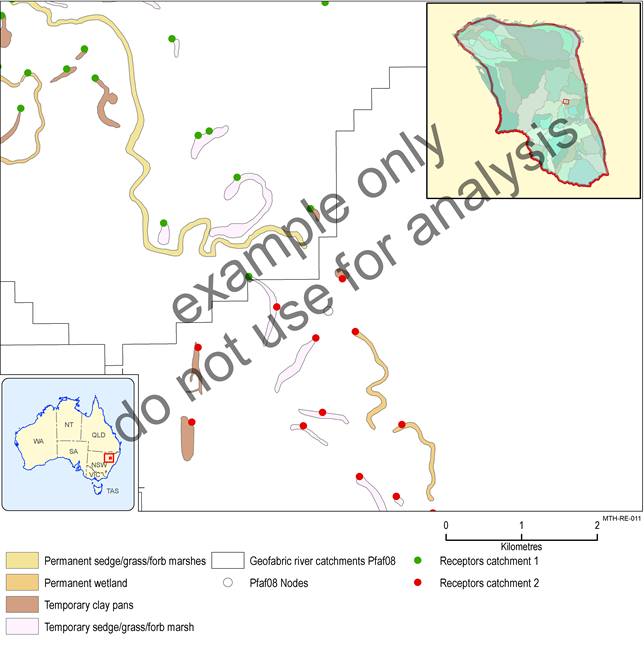
Figure 12 Example of the distribution of surface water receptors in the Namoi subregion
In this example, a receptor is placed within each landscape class polygon at the location closest to the nearest downstream Pfafstetter river basin node.
Data: example data derived from Bureau of Meteorology (Dataset 1) and SEWPaC (Dataset 2)
