10.1 Outputs for product 2.6.2 (groundwater numerical modelling)
Product 2.6.2 (groundwater numerical modelling) reports the potential impacts of coal resource development on water resources at the selected model nodes within the groundwater model domain. This is done by comparing model simulations that account for the coal resource development pathway (CRDP) with those that only consider the baseline.
10.1.1 Hydrological response variables
The groundwater modelling outputs hydrological response variables, the hydrological characteristics of the system or landscape class that potentially change due to coal resource development. These outputs from the groundwater modelling can be either fluxes or stores. They need to be decided before the sensitivity analysis begins and also need to be defined precisely ‒ for example, drawdown at location (x, y, z) at time t.
The primary hydrological response variables for groundwater are shown in Table 4.
Table 4 Primary hydrological response variables for groundwater
Figure 15 shows an example of output for hydrological response variables for the Clarence-Moreton bioregion (see Cui et al. (2016) for full explanation and interpretation of these results). Uncertainty analysis has been undertaken for these results as well (as per Chapter 8).
Other outputs from groundwater modelling include:
- groundwater fluxes to or from the stream network, which are fed back to the surface water modelling (Viney, 2016) and are reported as surface water hydrological response variables in product 2.6.1 (surface water numerical modelling)
- the volume of co-produced water and mine water make, which is reported in product 2.5 (water balance assessment)
- interpolated surfaces of percentiles of drawdown and probability of exceeding thresholds of 0.2 and 2 m for the baseline, CRDP and additional coal resource development.
Some groundwater models will be capable of generating many gigabytes of output data from a single model run. When such models are run thousands of times, the storage space required may become infeasible and file transfers may become prohibitive or impossible. For this reason, only the model outputs that will actually be used in evaluating the potential impacts of coal resource development on assets and landscape classes will be stored.
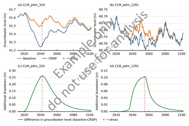
Example only; do not use for analysis. This is an early draft of a figure published in Cui et al. (2016). See Cui et al. (2016) for full explanation and interpretation of these results.
Additional drawdown is the maximum difference in drawdown (dmax) between the coal resource development pathway (CRDP) and baseline, that is due to additional coal resource development
Coal resource development pathway = baseline + additional coal resource development
10.1.2 Content for product 2.6.2 (groundwater numerical modelling)
Table 5 shows the recommended content for product 2.6.2 (groundwater numerical modelling).
The outline for product 2.6.2 (groundwater numerical modelling) can be flexibly adapted where there are multiple groundwater models. There are several reasons why there could be multiple groundwater models within a subregion or bioregion including:
- where the development occurs in two distinct geographical regions without overlap
- a hybrid approach with models feeding in to one another, or
- if child models are used for detail in an area of a regional model.
In the Bioregional Assessment Technical Programme only the Gloucester subregion has multiple groundwater models. Two models were built for the Galilee subregion, although only one is used directly for the Bioregional Assessment Technical Programme analysis.
Table 5 Recommended content for product 2.6.2 (groundwater numerical modelling) when there is one groundwater model
|
Section number |
Title of section |
Main content to include in section |
|---|---|---|
|
2.6.2.1 |
Methods |
Summary This section identifies the models used, the interactions between the different models, the sequence in which they need to be run and for which model nodes they simulate the impact of coal resource development. |
|
2.6.2.2 |
Review of existing models |
Summary This section reviews the previous groundwater models developed for coal resource development in the subregion or bioregion. Level 5 headings can cover individual projects. |
|
2.6.2.3 |
Model development |
Summary This section describes how the model was developed. The following Level 5 headings are recommended but not mandatory. 2.6.2.3.1 Objectives 2.6.2.3.2 Hydrogeological conceptual model 2.6.2.3.3 Design and implementation 2.6.2.3.4 Model code and solver 2.6.2.3.5 Modelling approach |
|
2.6.2.4 |
Boundary and initial conditions |
Summary This section characterises the boundary and initial conditions. The following Level 5 headings are recommended but not mandatory. 2.6.2.4.1 Lateral 2.6.2.4.2 Recharge 2.6.2.4.3 Surface water – groundwater interactions |
|
2.6.2.5 |
Implementation of coal resource development pathway |
Summary This section describes how the coal resource development pathway (as specified in product 2.3 (conceptual modelling)) is implemented in the groundwater model. The following Level 5 headings are recommended but not mandatory. 2.6.2.5.1 Open-cut mines 2.6.2.5.2 Underground mines 2.6.2.5.3 Coal seam gas wells |
|
2.6.2.6 |
Parameterisation |
Summary Table 6 (in this submethodology) provides an exemplar table for listing parameters in this section. |
|
2.6.2.7 |
Observations and predictions |
Summary This section provides the results, namely predictions of the hydrological response variables and the sensitivity of the results to the parameters used. The following Level 5 headings are recommended but not mandatory. 2.6.2.5.1 Predictions 2.6.2.4.2 Sensitivity analysis |
|
2.6.2.8 |
Uncertainty analysis |
Summary Both qualitative and quantitative uncertainty is presented. 2.6.2.6.1 Qualitative uncertainty analysis The qualitative uncertainty analysis lists the main model assumptions and choices and discusses their potential effect on the predictions. Table 7 (in this submethodology) provides an exemplar table. 2.6.2.6.2 Quantitative uncertainty analysis For the quantitative uncertainty analysis, prior distributions, including covariance, are specified for all parameters from expert elicitation; constraining these prior distributions with the maximum coal seam gas (CSG) and coal mine water production rate results as well as head and flux observations in posterior probability distributions for dmax and tmax. The potential effect on the predictions are discussed along with a comparison to previous model results. Figure 16 and Figure 17 (in this submethodology) provide exemplar figures. |
|
2.6.2.9 |
Limitations and conclusions |
Summary This section describes the use for which the groundwater model was developed, and limitations on its application to other uses. |
Table 6 Example table to include in Section 2.6.2.6: parameters of the Avon and Karuah models for the Gloucester subregion
Example only; do not use for analysis
The ‘value’ column lists the initial parameter value simulation, while the ‘minimum’ and ‘maximum’ columns show the range sampled for the design of experiment. The last two lines list non-variable parameters used in the simulations.
na = not applicable
See Peeters et al. (2016) for full explanation and interpretation of these results.
Table 7 Example table to include in Section 2.6.2.8: qualitative uncertainty analysis as used for the Gloucester subregion
Example only; do not use for analysis.
CSG = coal seam gas
See Peeters et al. (2016) for full explanation and interpretation of these results.
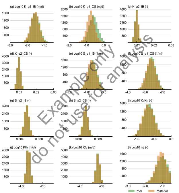
Example only; do not use for analysis.
The extent of the x-axis in each plot corresponds to the range of parameters sampled during the design of experiment. Refer to Table 3 in Section 2.6.2.3.4 for definitions of terms.
See Peeters et al. (2016) for full explanation and interpretation of these results.
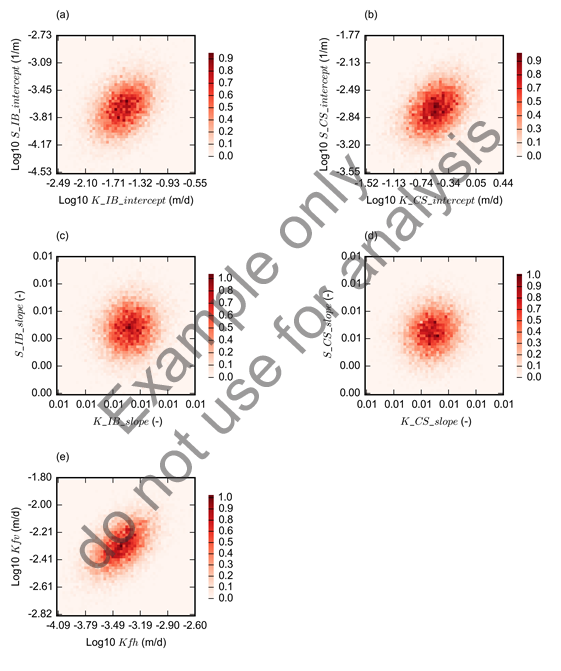
Example only; do not use for analysis.
The colour scale is proportional to the density of points. Refer to Table 5 in Section 2.6.2.6 of Peeters et al. (2016) for definition of terms. See Peeters et al. (2016) for full explanation and interpretation of these results.
10.2 Outputs for product 2.5 (water balance assessment)
Product 2.5 (water balance assessment) presents a quantitative water balance for the subregion. The groundwater components of this water balance are typically derived from the outputs of the groundwater modelling. Other approaches for determining groundwater balance components may be required (e.g. SKM, 2006) if the groundwater modelling undertaken for a subregion does not provide the necessary information for reporting in the water balance. Table 9 shows the recommended content for product 2.5 (water balance assessment).
The water balance will represent a defined control volume. The nature of this control volume may vary between subregions or bioregions. However, it is likely to involve a subarea of the surface water model domain. It may represent a hydrologically intact catchment area (or areas) draining to a particular point (or points) in the river network, or it may exclude external tributary inflows. Since there will be a groundwater component to the water balance, the extent of the control volume may be constrained by the spatial extent of the groundwater model. In other words, it is likely that the control volume will be a subarea of the intersection between the spatial domains of the surface and groundwater models. In product 2.5 a map will be provided that shows the location of the control volumes used for the water balance.
The following groundwater components will be reported in the water balance:
- recharge
- evapotranspiration
- baseflow (discharge to stream)
- upward flow from deeper groundwater
- change in storage.
An exemplar for a water balance table is shown in Table 8 (see Herron et al. (2016) for full explanation and interpretation of these results).
Table 8 Example water balance table: mean annual groundwater balance for the alluvial groundwater model extent in the Avon River for 2013 to 2042 in the Gloucester subregion (ML/year)
Example only; do not use for analysis.
The first number is the median, and the 10th and 90th percentile numbers follow in brackets.
See Herron et al. (2016) for full explanation and interpretation of these results.
Table 9 Recommended content for product 2.5 (water balance assessment)
