The groundwater models used in the Bioregional Assessment Programme have a relatively simple parameterisation. That is the hydrostratigraphic layers are generally assumed to be homogeneous with the properties having a depth dependence and are modified due to geomechanical deformation following longwall mining.
7.1 Assumption of homogeneity of aquifer parameters
In most groundwater models developed for BA purposes, spatial heterogeneity of hydraulic properties is not represented explicitly. Most hydrostratigraphic units are assigned a spatially uniform hydraulic property.
This section illustrates that by stochastically varying this uniform hydraulic property, the variation in predicted groundwater levels is at least as large as the variability that would arise from simulating spatial heterogeneity explicitly. This means that the stochastic predictions will be conservative (i.e. the range of the ensemble prediction will be larger compared to the range based on modelling heterogeneous hydraulic properties).
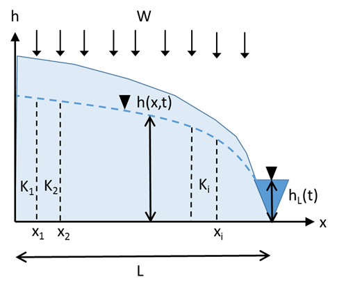
Figure 10 Conceptualisation of groundwater flow example (after Liang and Zhang, 2013)
The steady state solution for the groundwater level at a distance ![]() from a no flow boundary, with a constant head boundary at
from a no flow boundary, with a constant head boundary at ![]() with constant head
with constant head ![]() , a spatially uniform diffuse recharge
, a spatially uniform diffuse recharge ![]() and piecewise constant, spatially varying hydraulic conductivity
and piecewise constant, spatially varying hydraulic conductivity ![]() for
for ![]() can be expressed as (Figure 10 and equations 4 and 5 in Liang and Zhang, 2013):
can be expressed as (Figure 10 and equations 4 and 5 in Liang and Zhang, 2013):
|
|
(7) |
|
|
|
(8) |
|
These equations present a linear approximation to groundwater flow in a spatially variable field and yields the same results as a numerical model that is discretised in ![]() grid cells. While this is a simplification of any field conditions, this general conceptual model resembles situations that are relevant to BA, such as groundwater mounding away from a river or groundwater level variation away from a mine that is drained to a fixed level.
grid cells. While this is a simplification of any field conditions, this general conceptual model resembles situations that are relevant to BA, such as groundwater mounding away from a river or groundwater level variation away from a mine that is drained to a fixed level.
Equations 7 and 8 are straightforward to implement numerically and are solved very quickly, which allows the exploration of the effects of spatial heterogeneity on groundwater level predictions.
Consider the log of hydraulic conductivity is normally distributed with a mean of 1 m/d and a standard deviation of 1:
|
|
(9) |
The spatial correlation can be described with an exponential variogram with correlation length ![]() so that the variance between two locations a distance
so that the variance between two locations a distance ![]() apart is:
apart is:
|
|
(10) |
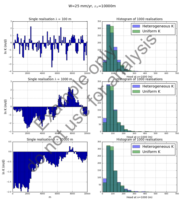
Figure 11 shows the results of a comparison of groundwater levels predicted at a distance of 9000 m from the constant head boundary (x=1000 m). For the heterogeneous case, 1000 samples of ln(K) are generated from a multivariate normal distribution with mean equal to zero and a covariance governed by equation 10 with three different correlation lengths (100 m, 1000 m and 10,000 m). For the uniform K case, 1000 samples of ln(K) are taken from the normal distribution specified in equation 9. The latter approach is the approach that is taken in the stochastic sampling in the uncertainty analysis of BA groundwater models.
From Figure 11 it becomes clear that the resulting ensembles of groundwater level predictions are nearly identical between the heterogeneous and the uniform hydraulic conductivity fields for the three different correlation lengths.
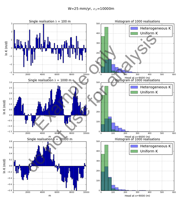
Figure 12 shows the same analysis for groundwater level predictions 1000 m from the constant head boundary (x=9000 m). It is apparent that the uniform hydraulic conductivity field results in ensembles that have a similar mean and median to the heterogeneous case, but the spread in the distribution is underestimated. This effect is more pronounced for short correlation length.
While this is by no means a comprehensive study of the effects of spatial heterogeneity on groundwater level predictions, some general findings are:
- At regional scale, i.e. distances larger than a few kilometres, from a stress or boundary condition, spatial heterogeneity has little influence on groundwater level predictions. The uncertainty in groundwater level predictions can be captured by stochastically varying a spatially uniform hydraulic conductivity
- At a local scale, i.e. distance smaller than a few kilometres from a stress or boundary condition, spatial heterogeneity will have a distinct effect on groundwater level predictions. The differences between simulating spatial heterogeneity and varying a spatially uniform hydraulic conductivity increase for decreasing correlation length (i.e. higher spatial variability).
Example only; do not use for analysis
Example only; do not use for analysis
7.2 Depth dependence of hydraulic properties
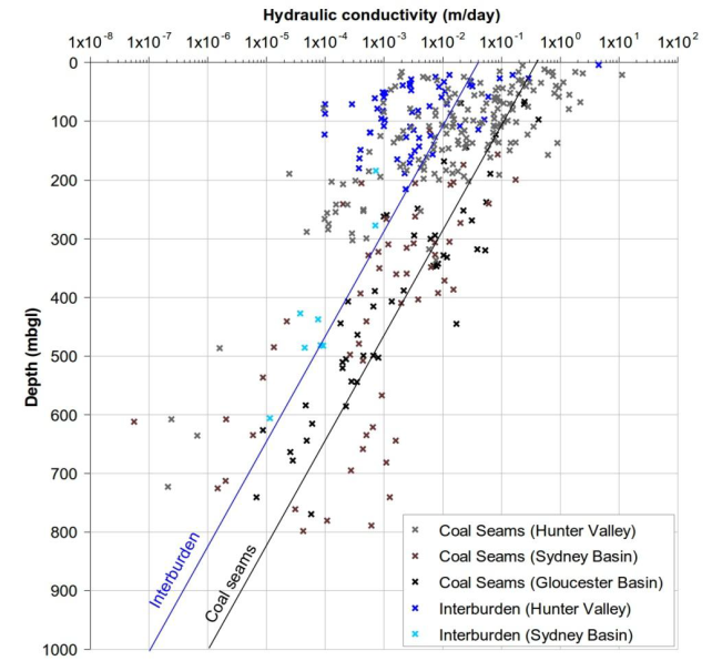
Even though a simple parameterisation of the models is used that will generally see hydrostratigraphic layers treated as homogeneous, the hydraulic properties used in the groundwater modelling have a depth dependence that has been observed in many coal basins. An example is shown in Figure 13 for data from the Hunter subregion, Gloucester subregion and Sydney Basin bioregion (Parsons Brinkerhoff, 2015).
Figure 13 Relationship between depth and hydraulic conductivity for coal seams and interburden
Source: Figure 7.3 in Parsons Brinckerhoff (2015). This figure is not covered by a Creative Commons Attribution Licence, it has been reproduced with the permission of AGL.
7.3 Changes in hydraulic properties post-mining
Following longwall mining there are often changes in hydraulic properties observed due to geomechanical deformation. This can be represented in the groundwater models by enhancing the hydraulic conductivity after longwall mining. The hydraulic conductivity, K, above and below each mine working, is enhanced according to:
|
(11) |
where K0 is the base conductivity (both horizontal and vertical components), and ![]() parameterises the conductivity change.
parameterises the conductivity change. ![]() before mining of the seam commences, and
before mining of the seam commences, and ![]() at height, h, above the seam after mining commences.
at height, h, above the seam after mining commences. ![]() is calculated using the following piecewise-linear function of the height above the mining seam, h:
is calculated using the following piecewise-linear function of the height above the mining seam, h:
|
(12) |
||||
|
(13) |
||||
|
|
(14) |
|||
| |
(15) |
|||
The general form of the relationship is illustrated in Figure 14 where it is clear that conductivity change is M orders of magnitude directly above the seam, and m orders of magnitude directly below the seam, and that the conductivity changes occur between -z below the seam and Z above the seam.
As discussed in Adhikary and Wilkins (2012), the effective conductivity in the immediate roof of longwall mines can be enhanced by up to 10 orders of magnitude. The enhancement of hydraulic conductivity can extend up to 500 m above and 250 m below the longwall panel.
METHODOLOGY FINALISATION DATE
- 1 Background and context
- 2 Modelling philosophy
- 3 Choice of model
- 4 Boundary conditions
- 5 Model time steps and predictive time frame
- 6 Integration with surface water modelling
- 7 Parameterisation
- 8 Calibration, sensitivity analysis and uncertainty analysis
- 9 Meeting the requirement for transparency
- 10 Outputs from groundwater modelling
- References
- Glossary
- Citation
- Acknowledgements
- Contributors to the Technical Programme
- About this submethodology

