Receptor impact models translate predicted changes in the hydrological regimes that help maintain landscape classes into predicted changes in one or more ecosystem variables. The regional landscape-level scope of the BA, however, provides for many choices during this process, whilst the complexity of the assessment combined with the time and resource limitations imposed on expert participation place many restrictions on what can be practically achieved within the time available for the BA. This section presents the set of criteria and processes that can be used to progress cumulative impact assessments for receptor impact variables.
The two most important choices during the receptor impact modelling are:
- hydrological response variables. The BA groundwater and surface water models could be used to predict many different characteristics of the hydrological regimes that operate in a landscape class, but these will not be equally important in maintaining and shaping the ecosystem. The choice of hydrological response variables to include in the receptor impact models should be guided by the results of the IMEA hazard analysis (see companion submethodology M11 (as listed in Table 1) for hazard analysis (Ford et al., 2016)), the capabilities of the surface water and groundwater models, and most importantly the hydrological variables identified by ecological experts when the signed digraphs of the landscape class are created.
- receptor impact variables. Typically, there are hundreds to thousands of assets identified within a BA bioregion or subregion and tens of variables identified within the sign-directed graphs of the landscape classes, with ecological assets either explicitly recognised as a model variable, or encompassed within a broader functional group. For example, a particular species of bird (the asset) may be encompassed within a function group of nocturnal predators. Given that expert participation is required to construct each receptor impact model, by necessity the receptor impact model process can only construct a few receptor impact models per landscape class, which accommodates no more than a few receptor impact variables per landscape class.
The choice of hydrological response variables ultimately will be a compromise between verbal descriptions of the hydrological regimes given by ecologists during the construction of the landscape class signed digraphs, and the numerical indices that are produced by the surface water and groundwater models. In this context it is important to recognise that the outputs of the surface water and groundwater models are typically finalised before the qualitative modelling workshops are conducted, and hence the model outputs are not specifically designed to address the hydrological regimes that are subsequently described. In most instances, however, the surface water and groundwater outputs are either directly relevant, or provide a sufficient basis to construct, the hydrological variables identified and verified by the expert ecologists as critical to the landscape class ecosystems.
The choice of receptor impact variables is framed by the complexities of the potential direct and indirect effects associated with press perturbations and the BA’s expected audience. There will be a wide range of interests represented across the Independent Expert Scientific Committee on Coal Seam Gas and Large Coal Mining Development (IESC, after 27 November 2012), regulators, industry and community. There will be experts in particular taxa and experts about particular locations. There will be experts about particular agricultural or ecological systems. Furthermore, many readers of the assessments will be members of the general public who will each have their own beliefs and understandings of these systems, and an associated set of values.
The Bioregional Assessment Programme (the Programme) and the Assessment team need to be conscious of the expectations of this community, and the natural tension that arises between ensuring that the risk analysis is achievable (within operational constraints) but at the same time relevant to as much of the community as possible. This can be achieved, for example, by choosing impact variables that simplify the elicitation task, by speaking to broad sections of the community, and by using narrative in the analysis to broaden the relevance of the assessment to other more specific sections of the community. For example, basal vegetation variables are relevant to diverse segments of the expected audience when interpreted in terms of forest cover and such.
To navigate the choice across the large set of possibilities, the BA approach is to adopt a selection process that is efficient and consistent across the Programme, and leads to effective and efficient communication to stakeholders. For example, choosing a cryptic species with unknown relationships to overall environmental health would be inefficient and potentially misleading. Impact variables that are identified as representative of core stakeholder and community values within that bioregion or subregion will be central to the assessment. Impact variables that are more directly and unambiguously connected to the hydrological response, and that are measurable in some sense will lead to more certain and useful receptor impact models. Impact variables that strongly speak to the condition or abundance of other components of the system are also clearly advantageous. For example, if the status of river red gums also informs about the health of other floodplain trees and organisms, then it is a good choice.
To assist in these considerations the BA developed the following selection criteria to help guide the choice of impact variable:
- Is the response variable directly affected by changes in hydrology? These variables typically have a lower trophic level, and focusing on direct (signed digraph arcs of length one) impacts helps alleviate the elicitation burden imposed on experts during the construction of the receptor impact models.
- Is its status important in maintaining other parts of the landscape class? Variables (or nodes) within the qualitative model that other components of that ecosystem or landscape class depend on will speak more broadly to potential impacts. Again, these types of variables will typically have a lower or mid-trophic level.
- Is it something that the available expertise can provide an opinion on? There is a need to be pragmatic and make a choice of receptor impact variable that plays to the capabilities and knowledge base of the experts that are available at the time the receptor impact models are created.
- Is it something that is potentially measurable? This is essential for (in)validation of the predicted impacts and in the subsequent design of monitoring strategies that close the risk analysis loop by testing, comparing its predictions with observations.
- Will the community understand and accept the relevance and credibility of the receptor impact variables for a given landscape class? This reflects the communication value of the receptor impact variable.
The challenge in applying these selection criteria is that a priori it is unlikely that any single impact variable will simultaneously satisfy all criteria. Examples of ecological variables that are likely to perform well when judged against these criteria include: the percent cover of a dominant canopy-forming species or plant association, the abundance or biomass of an iconic species, or the abundance/biomass of a particular key functional group (e.g. invertebrate food source for waterbirds and other predators).
The importance of a dominant canopy-forming species or plant association is reflected in its key role in forming habitat for other species. It is also likely to have a low trophic level and therefore be directly impacted by changes in hydrological variables and a major change in the component of the ecosystem will likely be noticed by the non-expert and casual observer alike. Iconic species are recognisable to large numbers of people and would reflect community concerns about particular changes but some life stages may be relatively insensitive to hydrological change. Changes in the abundance or biomass of key prey groups (such as aquatic invertebrates) are again likely to be relatively low in the food chain and potentially more proximal to hydrological changes, and also be important in maintaining many other groups within the ecosystem, for example iconic predators such as the platypus (Ornithorhynchus anatinus), and hence are more easily aligned with ecological features of the landscape class that are valued by the community.
To illustrate the potential choices, complexities and the implications the choice of impact variable holds for the estimation of direct and indirect effects, the Assessment team can identify three impact scenarios of increasing complexity:
- Press perturbation involving only a single hydrological response variable, which leads only to direct impacts (i.e. single link in causal pathway). In this most simple scenario, the outputs from the coal resource development pathway (CRDP), the hazard analysis, and signed digraph (stressor conceptual model) predict only direct impacts between an individual hydrological response variable and receptor impact variable. The quantification of the impact proceeds by eliciting the expected change in the receptor impact variable (y‑axis in the figure on right-hand side of Figure 8) conditional on the change in hydrological response variable (x-axis in the figure on the right-hand side of Figure 8), via the scenario creation and receptor impact modelling process. Note this scenario is shown here for illustrative purposes only and may never occur in reality.
- Press perturbation to a single hydrological response variable, leading to direct and indirect impacts. In this more complex situation, the signed digraph may indicate the existence of both direct and indirect causal pathways leading from the hydrological response variable to the receptor impact variable of interest. In Figure 9, the indirect pathways from FR3 to HF MI involve additional intervening variables. In this example not only is there a choice of receptor impact variable, but, if an interest in HF MI is maintained, the quantification of the direct and indirect effects on HF MI must either be explicitly accounted for in the statistical model (an option not practical given the time and resource limitations imposed on expert participation) or the expert must be asked for the predicted change in HF MI averaging over the possible changes in the intervening variables.
- Press perturbations to multiple hydrological response variables, leading to direct and indirect impacts on multiple potential receptor impact variables. In this more complex but realistic scenario, the signed digraph identifies direct and indirect impacts on multiple receptor impact variables arising from simultaneous press perturbations to multiple hydrological response variables (Figure 10). The complexity of this process can be described in the scenario creation step prior to the receptor impact modelling, but again there is a choice of receptor impact variable, and, if an interest in variable WRV is maintained, the expert must account for the effects of FR1 and FR2 on Seedl, and their indirect impact on WRV as well as the direct effects of FR1, FR2 and GW on WRV. The statistical model leads to a response surface that allows for interactions and non-linear relationships between the expert response and the hydrological response variables.
By representing stressor conceptual models as sign-directed graphs (see Chapter 3), the BA methodology is able to make qualitative predictions of long-term, press perturbation impacts to variables (i.e. direction but not magnitude of change) in the landscape class stressor conceptual model. This facet of the analysis provides the possibility of comparing the predicted direction of change of the qualitative mathematical analysis with the quantitative analysis of the receptor impact variable, and also provides whole-of-system qualitative predictions for the landscape class that may be informative during the post-assessment monitoring, in addition to the quantitative predictions available from the receptor impact model analyses. The sign-directed graphs were constructed from expert participation within the qualitative modelling workshop (Figure 4).
In conjunction with input from the hydrological modelling, the sign-directed graph in turn advised the design of the quantitative receptor impact modelling workshop (Figure 4). The quantitative receptor impact model predicts the magnitude of the receptor impact variable response given changes in the identified hydrological response variables (Figure 8, Figure 9, Figure 10). The quantitative receptor impact model additionally captures not only long-term responses to press perturbations but also potentially transient responses to pulse perturbations. The quantitative receptor impact model quantifies the uncertainty in the response of the receptor impact variable due to uncertainty in the direct impacts, indirect impacts and other factors or pathways that are not explicitly represented. It is important to recognise that the risk methodology proposed here is capable of quantifying the direct impacts under scenario 1, and direct and indirect impacts under scenarios 2 and 3 including the case where these are mediated by indirect effects, but the elicitation task is made increasingly more difficult through scenarios 2 and 3. As noted in the above discussion, it is a matter of choice on what factors to explicitly include within a quantitative receptor impact model. Whereas including more factors or hydrological response variables may seem more comprehensive, the cost of the increased complexity is that a more elaborate and complicated model that could increase the difficulty of an elicitation is required. For example, fundamental relationships among identified water availability metrics and the receptor impact variable could be obscured by additionally conditioning on intermediary variables.
In practice, the BA seeks to minimise the complexity of the analysis by judicious choice of hydrological response variables and receptor impact variables so that, wherever possible (and acceptable to managers and stakeholders), the analysis is constrained to receptor impact modelling within scenario 1. Where this is not possible, the elucidation of the system framework in the graphical depiction of the sign-directed graph can help the expert allow for different alternative pathways while contributing their assessment.
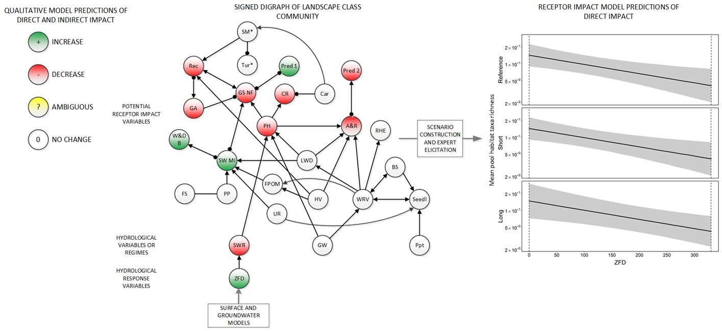
The schematic shows the simplest impact scenario focused on a particular receptor impact variable within a landscape class community. In this scenario, a decrease in hydrological variable surface water replenishment (SWR) is modelled as an increase in hydrological response variable zero-flow days (averaged over 30 years) (ZQD). Under the stressor conceptual model (represented here by the sign-directed graph) this is deemed to have a direct impact on the receptor impact variable Invertebrate Taxa within Pool Habitat (PH). The signed digraph also provides qualitative predictions (node colours) of the (long-term) knock-on effects through the ecosystem on to other variables. The impact of this direct effect is quantified through the receptor impact model (right-hand panel). The receptor impact model (essentially a generalised linear model with expert opinion as data) predicts how the median value of the receptor impact variable changes in response to changes in the hydrological response variable (HRV; black line in right-hand plots) together with the uncertainty associated with these predictions (grey polygons in the right-hand plot), for the reference (2012), short (2042) and long (2102) assessment years. Note that all self-effects are omitted from the sign-directed graph for clarity. Dashed vertical lines on the right-hand panels show the minimum and maximum HRV values provided to the elicitation team prior to the receptor impact modelling workshops. This scenario is shown for illustrative purposes and may never occur in reality. Readers should refer to the ‘Intermittent – gravel/cobble streams’ landscape class in companion product 2.7 for the Gloucester subregion (Hosack et al., 2018) for further information on the nodes shown in the signed digraph.
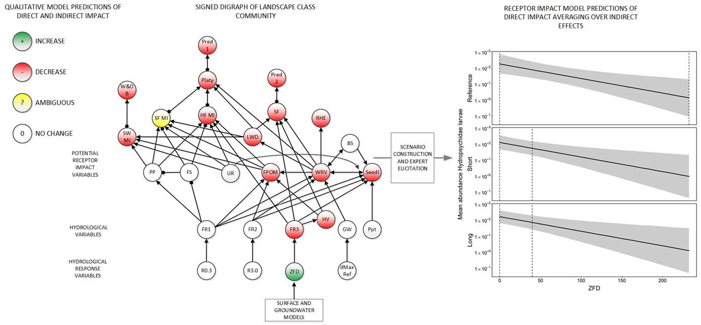
In this scenario, the development’s impact on the hydrological variable flow regime 3 (FR3) is modelled as a decrease in the hydrological response variable zero-flow days (averaged over 30 years) (ZQD) for another landscape class. Under the stressor conceptual model this has a direct impact on receptor impact variable high-flow macroinvertebrates (HF MI), where increasing zero-flow days corresponds to decreasing abundance of HF MI, but it also impacts herbaceous vegetation (HV) which influences fine organic particulate matter (FPOM), and woody riparian vegetation (WRV through seedlings) which provide habitat to platypus (Platy) that consume HF MI. The direct and indirect impact on receptor impact variable (the abundance of Hydropsychidae larvae) caused by changes in ZQD is quantified in the receptor impact model. In this situation the model must either explicitly account for the indirect interactions of ZQD on HF MI as mediated by FPOM and Platy, or the expert must account for the direct and indirect interactions internally during the elicitation by marginalising over the indirect pathways from ZQD as mediated by FPOM and Platy. The receptor impact model (essentially a generalised linear model with expert opinion as data) predicts how the median value of the receptor impact variable changes in response to changes in the hydrological response variable (HRV; black line in right-hand plots) together with the uncertainty associated with these predictions (grey polygons in the right-hand plot), for the reference (2012), short (2042) and long (2102) assessment years. Note all self-effects are omitted from the sign-directed graph for clarity. Dashed vertical lines on the right-hand panels show the minimum and maximum HRV values provided to the elicitation team prior to the receptor impact modelling workshops. Readers should refer to the ‘Perennial – gravel/cobble streams’ landscape class in companion product 2.7 for the Gloucester subregion (Hosack et al., 2018) for further information on the nodes shown in the signed digraph.
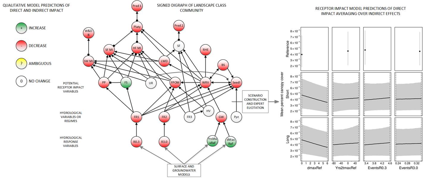
In this scenario, the development simultaneously changes hydrological variables flow regime 1 (FR1), flow regime 2 (FR2) and groundwater depth (GW). These changes are modelled as decrease in hydrological response variables Events R0.3 (R0.3) and Events R3.0 (R3.0), and an increase in hydrological response variable maximum groundwater depth relative to the reference period (dMaxRef) and years to maximum groundwater depth (YrsMaxRef). Under the stressor conceptual model this leads to direct impacts on receptor impact variables wood riparian vegetation (WRV), fine sediment (FS), primary production (PP) and fine particulate organic matter (FPOM). To quantify the direct and indirect impacts of the hydrological response variables on WRV in this instance, the model must either explicitly account for the direct effect of FR1 and FR2 on the additional ecological variable seedlings (Seedl) and its indirect interaction with WRV, or the expert is asked to marginalise over the direct and indirect effects during the elicitation. In this case the plot on the right-hand side shows how the median value of the receptor impact variable changes in response to changes in these hydrological response variables (HRV; black line in right-hand plots) together with the uncertainty associated with these predictions (grey polygons in the right-hand plot), holding all other hydrological response variables at their median values, for the reference (2012), short (2042) and long (2102) assessment years. Note all self-effects are omitted from the sign-directed graph for clarity. Dashed vertical lines on the right-hand panels show the minimum and maximum HRV values provided to the elicitation team prior to the receptor impact modelling workshops. Readers should refer to the ‘Perennial – gravel/cobble streams’ landscape class in companion product 2.7 for the Gloucester subregion (Hosack et al., 2018) for further information on the nodes shown in the signed digraph.
