4 Methodology

Figure 8 outlines the methodology for propagation of uncertainty within the BA. The main process, in blue, starts with the compartmentalisation of the conceptual model (i.e. subdividing the conceptual model into a number of sub-models without feedback loops). For each of these sub-models a comprehensive and robust sensitivity analysis is subsequently carried out to identify the model factors (parameters and assumptions) that have the largest impact on the hydrological response variables of interest. From this factor prioritisation, a relatively small number of factors will be selected for inclusion in the actual uncertainty analysis, which will result in a probability distribution function (pdf) for the hydrological response variable (or metric) of interest. When carried out sequentially for each sub-model in the model chain, the process will culminate in the probability distribution function of the hydrological response variable. Since the model chain is compartmentalised, the uncertainty is additive.

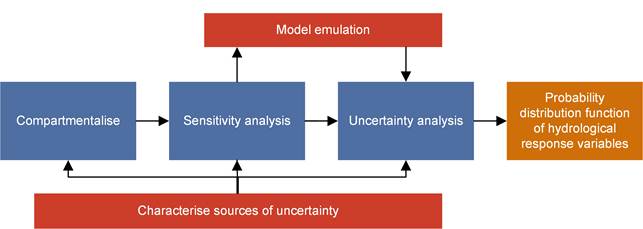
Figure 8 Uncertainty methodology flowchart

Blue boxes indicate the main workflow, the orange box is the result of the workflow and the red boxes indicate concepts and methods that are essential to complete the workflow

At this point it is worthwhile to clearly define and differentiate between the interlinked notions of sensitivity analysis and uncertainty analysis. Saltelli et al. (2008) differentiate between the two as follows:

Uncertainty analysis is the quantification of uncertainty. Sensitivity analysis is the study of how uncertainty in the output of a model (numerical or otherwise) can be apportioned to different sources of uncertainty in the model input.

An important goal for a BA is, where possible, to carry out an uncertainty analysis to quantify the uncertainty in the prediction of the effect of coal resource development. Sensitivity analysis will provide insight in how the different sources of uncertainty interact and, at least in this methodology, will primarily be used to focus the effort of the uncertainty analysis on the factors that contribute most to the uncertainty in the prediction.

The two red boxes in Figure 8 represent two crucial aspects of the methodology that will interact with the main process. The first of these is the characterisation of the sources of uncertainty, that is the identification of all possible sources of uncertainty and where possible the quantification of this uncertainty in probabilistic terms from observations or through expert elicitation. The second red interacting box is model emulation. The uncertainty analysis will require a very large number of model runs to arrive at a robust estimate of predictive uncertainty. Integrating each sub-model into uncertainty analysis software is challenging and for some BA models, runtimes will preclude running the model a sufficient number of times to arrive at a robust prediction. The methodology therefore opts to capture the dynamics between the key influential factors, identified through the sensitivity analysis, and the hydrological response variable of interest with a statistical model. It is this statistical model, the model emulator, which will be used for the actual uncertainty analysis. Model emulators are described in more detail in Section 4.5.

The reporting of the propagation of uncertainty through the models will be an integral part of the reporting on the hydrological and hydrogeological models (products 2.6.1 (surface water numerical modelling) and product 2.6.2 (groundwater numerical modelling)).

The following sections discuss in more detail each of the components of the flowchart depicted in Figure 8, beginning with more detail on the characterisation of the sources of uncertainty.

4.1 Characterisation of sources of uncertainty

Uncertainty arises in many aspects of the modelling process and there is a wide variety in the terminology used to describe the source and nature of uncertainty (Walker et al., 2003). Hayes (2011) summarises this varied terminology in the Venn diagram shown in Figure 9.

Decision uncertainty relates to the uncertainty that enters policy analysis after risks have been estimated. As such, this lies outside the scope for the BA. Linguistic uncertainty, however, is an aspect of uncertainty analysis that needs attention. It arises through communication about uncertainty using language that is not precise. Important aspects are vagueness, context dependence, ambiguity, indeterminacy and under-specificity (Hayes, 2011). Even when adopting clear mapping between numerical probabilities and linguistic terms, such as that used by the International Panel for Climate Change (IPPC) where for instance a probability between 90 and 100% is expressed as ‘Very Likely’ (see Mastrandrea et al., 2010), it has been shown that interpretation by policy makers and the general public is still very individual and context-specific (Spiegelhalter et al., 2011). Linguistic uncertainty will especially come into play when communicating the results of the uncertainty analysis (Patt, 2009) and during expert elicitation workshops (O’Hagan et al., 2006).

The focus of this submethodology report, however, is on variability and on epistemic uncertainty. Variability is the variation in a quantity or process that is caused by natural fluctuations or heterogeneities. Variability can be described in probabilistic terms, but cannot be reduced. Epistemic uncertainty lumps all uncertainty together that stems from incomplete knowledge, understanding or representation of the system under study. In theory, this form of uncertainty is reducible by gathering additional data and a more exact representation of the system in models. It is seldom possible to attribute uncertainty of a value solely to one or both types of uncertainty. The uncertainty in the hydraulic properties of an aquifer for instance is largely attributable to epistemic uncertainty, as generally there are only a few measurements of these properties. Even with unlimited resources, it would not be possible to deterministically describe the hydraulic properties due to natural heterogeneity of the subsurface (de Marsily et al., 2005; Caers, 2011) and so, part of the uncertainty in the hydraulic properties will remain due to variability.

Figure 9 Venn diagram illustrating four broad categories of uncertainty with more specific types of uncertainty (black) and different nomenclature (grey italic).

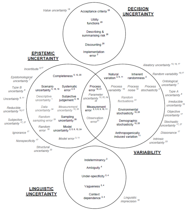
Source: Figure 2.3 in Hayes (2011). This figure is not covered by a Creative Commons Attribution licence. It has been reproduced with the permission of CSIRO. The numbers in superscript refer to references in that report.

Regardless of the source of uncertainty, the quality of the uncertainty propagation, such as presented in Figure 8, hinges on the characterisation of the uncertainty to be propagated. An adequate characterisation of an uncertain factor not only entails a quantitative aspect, in which the value, the units and the spread or variation are described, but it also needs to have a qualitative aspect (van der Sluijs et al., 2005). This qualitative aspect assesses both the quality of the information (e.g. the significance level of a statistical test) and whether the estimate is pessimistic or optimistic. The latter will generally be based on expert judgement, such as through a peer review.

The next three sections provide some guidance on how to characterise uncertainty in view of the above-mentioned philosophy. The discussion is differentiated based on two important practicalities:

4.1.1 Model assumptions

It is widely recognised that the assumptions and conceptual model choices that form the basis of any environmental model are crucial, albeit often overlooked, components of the uncertainty analysis (Saltelli and Funtowicz, 2014). In the field of hydrogeological modelling this is vividly illustrated in the classic paper by Bredehoeft (2005), where post-audits of several groundwater models revealed major shortcomings in conceptualisation.

Section 3.2.1 postulates that in this methodology every aspect of the model will be scrutinised while Section 3.1.3 states the requirement for the uncertainty analysis to be fully probabilistic. In a very practical sense, for a model aspect to be amenable for sensitivity analysis and uncertainty analysis, it needs to be able to be varied in an automated fashion through some sort of computer script. This obviously implies that all model aspects that cannot be varied automatically due to technical issues or other operational constraints cannot be part of the probabilistic uncertainty analysis.

Refsgaard et al. (2006) and Kloprogge et al. (2011) provide examples of methods to formally account for the uncertainty introduced by these kind of model assumptions. The pivotal aspects of these methodologies are the structured listing of model assumptions, and the analysis of the implications and influence of those assumptions (a pedigree analysis) through peer review or a workshop with experts and stakeholders. Finding and listing all key assumptions requires, as argued by Saltelli et al. (2013), an assumption-hunting attitude in order to ‘find important assumptions before they find you’. The pedigree analysis in Kloprogge et al. (2011) for instance suggests scoring each assumption on aspects such as the practical motivation, plausibility, availability of alternatives, agreement among peers and stakeholders and, most importantly, the perceived influence on the final prediction. While it is recognised that these scoring systems are prone to subjectivity and their results can be heavily influenced by the numerical scoring system used, such methods are very useful for a BA. The main benefit is that they provide a structured way of thinking about and analysing model assumptions which can help in the open and transparent communication of model uncertainty.

Section 2.6.2.8.2 (qualitative uncertainty analysis) in the Gloucester subregion groundwater model product (product 2.6.2, Table 2) shows an example of such a structured listing and discussion of model assumptions (Table 3).

Table 3 Qualitative uncertainty analysis as used for the Gloucester subregion

CSG = coal seam gas

The major assumptions and model choices underpinning the Gloucester groundwater models are listed in Table 3. The goal of the table is to provide a non-technical audience with a systematic overview of the model assumptions, their justification and effect on predictions, as judged by the modelling team. This table is aimed to assist in an open and transparent review of the modelling.

In the table each assumption is scored on four attributes using three levels; high, medium and low. Beneath the table, each of the assumptions are discussed in detail, including the rationale for the scoring. The data column is the degree to which the question ‘if more or different data were available, would this assumption/choice still have been made?’ would be answered positively. A ‘low’ score means that the assumption is not influenced by data availability while a ‘high’ code would indicate that this choice would be revisited if more data were available. Closely related is the resources attribute. This column captures the extent to which resources available for the modelling, such as computing resources, personnel and time, influenced this assumption or model choice. Again, a ‘low’ score indicates the same assumption would have been made with unlimited resources, while a ‘high’ value indicates the assumption is driven by resource constraints. The third attribute deals with the technical and computational issues. ‘High’ is assigned to assumptions and model choices that are dominantly driven by computational or technical limitations of the model code. These include issues related to spatial and temporal resolution of the models.

The final, and most important column, is the effect of the assumption or model choice on the predictions. This is a qualitative assessment of the modelling team of the extent to which a model choice will affect the model predictions, with ‘low’ indicating a minimal effect and ‘high’ a large effect. Especially for the assumptions with a large potential impact on the predictions, it will be discussed that the precautionary principle is applied; that is, the hydrological change is over- rather than underestimated.

4.1.2 Observation data

In a BA, a large amount of resources is invested in gathering and analysing existing data. These data will be used to inform the conceptual model. Some of these data will become part of the model chain as they inform models on initial conditions, boundary conditions and parameters. Section 4.4 will elaborate upon how observation data can be used to constrain the models.

The probability density for numerical, continuous variables can be described via the parameters of a probability density function. The most well-known is the normal distribution which is fully described by the mean and standard deviation. There is a wide variety of other types of distributions that can be used to describe a dataset. Uncertainty of categorical data can be expressed as a probability of occurrence of each category, where the total probability of all possibilities needs to sum to one.

Observations will always have a measurement uncertainty. The precision and accuracy of measurement devices is generally well-known and therefore straightforward to incorporate in the probability distribution. Larger contributors to measurement uncertainty are the location and time of measurement. For historical data and for subsurface data, the date of the measurement is often not recorded accurately and the elevation or the depth of the measurements are sometimes not available. Even when these are available, they can be of questionable accuracy. Another contributor to measurement error is the observation model used. River discharge for instance is mostly inferred from river stage elevation through a rating curve. The shape of this curve can contribute markedly to measurement uncertainty (Tomkins, 2014).

The data that will inform environmental models, however, will always have spatial and temporal support. This implies that point measurements of parameters and driving forces need to be upscaled to the scale relevant to the model, whilst model simulation results often need to be downscaled to be able to be compared with observations at a point scale. The spatial and temporal variability of data therefore also need to be described. Traditional techniques such as the variogram for spatial data and autoregressive–moving-average time series models for temporal data can be used to capture the spatio-temporal variability for stationary systems. Describing more complex variability is beyond the limitations of these simple hydrological response variables. In those cases, there is a need to resort to explicitly describing the variability through stochastic realisations of the spatial or temporal field. An example for rainfall grids is given in Shao et al. (2012).

Van Loon and Refsgaard (2005) provide an extensive overview of and guidance on assessing data uncertainty, with a focus on water resources management. It provides a good reference document for BAs as it provides detailed discussions on characterising uncertainty for meteorological, soil physical and geochemical, geological and hydrogeological, land cover, river discharge, surface water quality, ecology and socio-economic data.

4.1.3 Expert elicitation

In many cases there will be insufficient relevant data available to directly inform the uncertainty characterisation of a factor of interest. These cases need to rely on expert elicitation. Expert elicitation aims at capturing the scientific understanding of a process or a quantity in a probability distribution by questioning experts. In order for the obtained probability distribution to be reliable, the elicitation method needs to be transparent and reflect a consensus of the opinion of the scientific experts (O’Hagan et al., 2006).

Consider the scenario where expert elicitation is required to estimate the change in depth to watertable from a water extraction scenario at several locations and times. In direct elicitation, the panel of experts are asked to directly estimate the change in watertable. The response in depth to watertable, however, will depend on many site- and time-specific factors. Such direct elicitation will pose a high cognitive load on the expert. An alternative elicitation method is elaboration (O’Hagan, 2012) in which the elicitation focuses on a set of quantities that govern the process. An essential step in elaboration is to break down the process that leads to a quantity of interest in cognitively manageable chunks. In this example, rather than estimating the change in watertable at a location directly, focus can shift to quantities such as the distance to extraction, the hydraulic properties and hydrostratigraphy of the aquifer, proximity to surface water features or faults. As such this is not too different from the way piezometric surfaces traditionally have been created in data-poor areas, as recently illustrated in the updated watertable map for the Great Artesian Basin (Ransley and Smerdon, 2012). A more formal way is to use these elicited quantities in a groundwater model (i.e. eliciting the probability distribution functions of parameters of a groundwater model).

In indirect elicitation, the priors for the parameters of a linear model (Kadane et al., 1980) or generalised linear model (Bedrick et al., 1996; Garthwaite et al., 2013) are based on expert opinion of the predicted response at various combinations of the covariates. In ecology, this approach is used to elicit expert opinion on the spatial distribution of a species given a set of physical attributes, which may be spatially distributed, and thereby specify priors for a generalised linear model (Al-Awadhi and Garthwaite, 2006; Denham and Mengersen, 2007; Murray et al., 2009).

Even after elaboration and reduction of the elicitation problem to a manageable set of parameters or other quantities of interest, a number of possible cognitive biases can influence the elicitation process. For example, probabilities elicited from experts may suffer from overconfidence, anchoring to arbitrary starting values and the availability of the frequency of events in the memory of the expert. These cognitive restrictions and recommended remedies are discussed by Kadane and Wolfson (1998) and Kynn (2008), who document some rules of thumb for an analyst to adopt when eliciting expert opinion, such as eliciting percentiles or quantiles from an expert (e.g. as in O'Hagan, 1998, for a hydrogeological model). Elicitation methods based on an expert's opinion of statistical moments have been found to be less reliable (Garthwaite et al., 2005). The quantile or percentile method is adopted by available elicitation software (Low-Choy et al., 2009). Web-based, direct elicitation tools for univariate priors are available, such as ‘The Elicitator’ (Bastin et al., 2013) and ‘MATCH’ (Morris et al., 2014). The former focuses on documenting the elicitation process, whereas the latter provides a web-based interface to the SHELF software (Oakley and O'Hagan, 2010) and focuses on direct prior elicitation.

A consensus on how to mathematically accommodate expert opinion in a group setting has not yet been achieved. In fact, it is not altogether clear what it means to assimilate group expert opinion in a decision-making context (see Garthwaite et al., 2005). An alternative to model-based approaches for assimilating group opinion is to instead use behavioural approaches (Clemen and Winkler, 1999). A formal method of behavioural aggregation can be used, such as the Delphi-method that is commonly used in ecology (Kuhnert et al., 2010). Alternatively, a consensus prior may be developed through interaction among the individuals within a group of experts (O'Hagan and Oakley, 2004). The behavioural aggregation through interaction may be applicable where the opportunity for feedback and discussion among experts is allowed and encouraged.

4.2 Compartmentalisation of the conceptual model

A number of conceptual models are developed for each BA, including regional-scale conceptual models that synthesise the geology, groundwater, surface water and surface ecosystems. The conceptual model of causal pathways (the conceptual model) brings together a number of these conceptual models and describe the potential links between coal resource development and impacts to water resources and water-dependent assets. Ultimately, it is the goal of the BA to translate the conceptual model into a chain of numerical models to predict potential impacts to water resources and water-dependent asset at particular points in space and time with quantified uncertainty.

At a high level, a conceptual model will include the aspects shown in Figure 10; the development will affect the physical system which subsequently influences the ecological system which finally results in an impact to water-dependent assets. As long as the arrows in Figure 10 can be considered as one-way interactions, the conceptual model can be subdivided into isolated subsystems. Conceptual modelling should identify any important potential feedback loops between subsystems. If they exist then they either need to be incorporated into the model or noted as a watchpoint and a gap.

Even within these subsystems, there is potential to further subdivide, as shown in Figure 11 for the physical system.

The compartmentalisation of a system consists of delineating the subsystems and, especially important, identifying the point of interaction. This point of interaction is an observable quantity or model outcome that forms the output of one model and will be input to the linked model. The change in flow rate due to coal resource development for example can be the point of interaction between the physical system and the ecological system. It will be the outcome of the hydrological model and form the input for an ecological response function. Note that the ecological response function can combine several hydrological response variables. Similarly, the geological model can provide an estimate of fault probability at a location, which will feed into the hydrogeological conceptual model and ultimately into the groundwater model.

Figure 10 High-level compartmentalisation of conceptual model

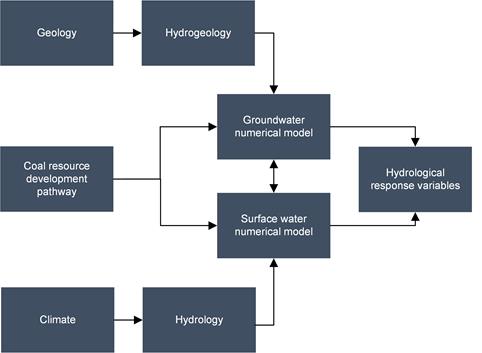
Figure 11 Example of compartmentalisation of the physical system

Conceptual representation of the physical system and inputs to and from the groundwater and surface water models. Surface water modelling uses the Australian Water Resources Assessment (AWRA) model suite, while the groundwater model varies between subregions and bioregions.

4.3 Sensitivity analysis for factor prioritisation

Sensitivity analysis (SA) methods can be broadly categorised into two groups, based on their strategy to explore parameter space: local SA and global SA. Local SA methods are usually based on the estimation of partial derivatives and provide measures of importance within a small interval around the ‘baseline’ or ‘nominal value’ point (Hill and Tiedeman, 2007; Doherty and Hunt, 2009; Nossent, 2012). Most local SA methods involve varying one model input factor at a time while keeping all others fixed, so they are special cases of ‘one-factor-at-a-time’ (OAT) approaches. An extensive review of these methods is provided in Turanyi and Rabitz (2000). Local SA methods are usually easy to implement and computationally cheap (require only a limited number of model evaluations), but are only suitable for linear or additive models. When these conditions are not satisfied, OAT approaches result in a sub-optimal SA due to the ignoring of the effect of interactions between input factors, since they do not take into account the simultaneous variation of input factors (Saltelli and Annoni, 2010).

Global SA overcomes the aforementioned drawbacks by exploring the full multivariate space of a model simultaneously. Since the 1990s, several global SA methods have been developed (Plischke et al., 2013): screening methods (Morris, 1991; Bettonvil and Kleijnen, 1997), non-parametric methods (Saltelli and Marivoet, 1990; Young, 2000), variance-based methods (Sobol, 2001; Saltelli et al., 2010; Nossent et al., 2011), density-based methods (Liu and Homma, 2009; Plischke et al., 2013), and expected-value-of-information based methods (Oakley et al., 2010). The last three categories require a larger investment in computer time, but they are more accurate and robust (Gan et al., 2014).

The main purpose of the sensitivity analysis in this methodology is to identify the subset of potential sources of uncertainty to which the hydrological response variables of interest are the most sensitive. This will allow for rationalising the uncertainty analysis and limiting its scope.

As outlined in Section 4.1.1, all factors of the model that can be changed automatically will be included in the sensitivity analysis and plausible ranges will need to be formulated for them. These are the ranges within which the factor will be varied to assess its influence on the outcome hydrological response variables. At this stage it is not essential that this range is the best estimate of the uncertainty of the factor; it is sufficient for the range to be plausible and realistic.

The ranges of each variable will be sampled in a quasi-random fashion using techniques such as Latin Hypercube sampling (Helton and Davis, 2003) or Sobol sampling (Sobol, 1976). Such sampling techniques generate random combinations of parameter values in an efficient way that maximises coverage of the range of each parameter and combination of parameters with a minimal number of samples.

Each of these samples (i.e. parameter combinations) is then evaluated using the original model and the model outcome is recorded. The number of model runs that will be carried out, however, will be equal to the number of model runs that are possible within the time allocated to this aspect of the project. It will depend on the model and the circumstances. As a rule of thumb, for a problem with a limited number of factors, less than 20, 1000 model runs are considered a minimum to ensure a minimal coverage of parameter space.

The analysis of the sensitivity analysis model runs will be done both qualitatively through visual inspection of scatter plots and quantitatively through sensitivity indices, where the sensitivity indices are preferably derived from a global SA method. The visual inspection of scatter plots of the variation of a factor against the model outcome hydrological response variable provides insight into the relationship between the factor and the hydrological response variable. Scatter plots are especially relevant to understand complex and non-linear model behaviour.

To objectively rank the factors, a quantitative measure of sensitivity is needed. Most of the above mentioned SA techniques provide such an objective measure.

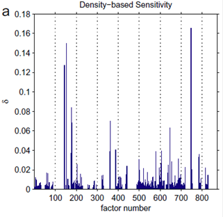
Figure 12 Sensitivity indices computed for a problem with 872 factors based on 65,000 model runs

Source: Figure 11a in Plischke et al., 2013. This figure is not covered by a Creative Commons Attribution licence. It has been reproduced with the permission of Elsevier.

As an example of the use of sensitivity indices, Figure 12 shows the result of an application of a density-based SA method, applied to a NASA space mission model (Plischke et al., 2013). The model has 872 uncertain factors and a single outcome. The model was run 65,000 times to assess the sensitivity of each factor. It becomes immediately apparent that there are only a limited number of factors that have a sizeable influence on the model outcome. This case study also illustrates that robust sensitivity estimates can be achieved for models with very high dimensionality with a limited number of model runs per parameter (~75 model runs per parameter in this case).

4.4 Uncertainty analysis is a function of data availability

The choice of uncertainty analysis methodology will be determined by the availability of relevant observation data. If no relevant observation data are available, the uncertainty analysis will be limited to a Monte Carlo simulation or propagation of the prior estimates of uncertainty of the important factors through the model chain. If relevant and sufficient data are available, the uncertainty analysis will be a Bayesian inference based on a Markov Chain Monte Carlo in which the observations will constrain the prior pdfs of the important factors to result in posterior pdfs of both the factors and the prediction.

Within the context of uncertainty analysis for BA, relevant observation data are data that are able to constrain the key influential factors that affect the model outcome hydrological response variable, as identified through the sensitivity analysis. A second condition is that the size of the dataset is sufficiently large to reliably constrain these factors. The evaluation of potential data starts with quality assessment to estimate the uncertainty of the observation data. From the sensitivity analysis described in the previous section, not only the effect of the factors on the prediction needs to be assessed, but also the effect of the factors on the model-simulated equivalents to the observation data. Observation data can only be considered relevant if its simulated equivalent is sensitive to parameters that are part of the subset of influential factors for the prediction of interest. Part of the evaluation of the observation dataset is to assess if the observation data are representative of the system or they are overly influenced by a local phenomenon. Related to this is the size of the dataset. Are there enough observations available to have a reliable estimate of the natural variability of the observations? If an observation dataset is considered not relevant for the uncertainty analysis, it does not mean that the data cannot be used within the BA uncertainty analysis. These data can still have potential to guide the expert elicitation of prior uncertainties of factors.

In the absence of sufficient relevant data, the prior probability distribution of each influential factor will be described, either from data or from expert elicitation. A Monte Carlo process will randomly sample these probability distributions and run these through the model. As such, this is the same as the sensitivity analysis process with the main difference being that the factors are no longer sampled uniformly from a plausible range, but from a distribution that reflects and incorporates the current knowledge on that factor. The resulting distribution of the prediction is then considered to be the estimate of uncertainty of the hydrological response variable.

When relevant data are available, the prior probability distribution of each influential factor will be described similar to the previous case. Rather than regular Monte Carlo simulation, Markov Chain Monte Carlo sampling will be applied. This sampling scheme favours parameter combinations that agree with the observation data. Several implementations of this scheme are available. A very promising tool is the LibBi software (Murray, 2013) developed by CSIRO, which is designed to maximally utilise the high-performance computing hardware available to BA.

4.5 Model emulation

The bottleneck in any Monte Carlo estimation is the large number of model runs required. Even for problems with moderate dimensionality, the number of simulations needed to arrive at robust estimates of the probability distribution function of the prediction will be in the order of 10,000 or even 100,000. For more complex models with higher dimensionality, millions of model runs might be required. Such large numbers of model runs are only feasible when the model run time is in the order of seconds. Most environmental models, however, take minutes, and in the case of groundwater models even hours, to converge to a solution.

Another potential bottleneck specific for BA is that each environmental model needs to be integrated into a software package or script that can carry out the Monte Carlo or Markov Chain Monte Carlo efficiently. The software implementation of environmental models likely to be used in BA can vary from straightforward spreadsheet calculations to custom-made scripts to third-party closed-source software. Implementing such a variety of software tools poses a significant challenge to the modellers and software engineers.

Both of these problems can be overcome using a technique called ‘model emulation’. The principle behind model emulation, sometimes referred to as surrogate modelling or meta-modelling, is to use a computationally efficient statistical approximation of the slower process-based model. Several techniques are available to create surrogate models (see Razavi et al., 2012). For BA, response surface models offer a relatively simple and well-studied solution to performing model emulation. In this technique, the response of a model to variations in the inputs and parameters is approximated with a mathematical function, such as a Gaussian Process (GP) model (O’Hagan, 2006) or Kriging (Kleijnen, 2009). The emulator is often implemented based on the output obtained from limited runs of the process-based model.

Of the statistical procedures used in model emulation, GP models are the most commonly utilised (see Kennedy and O’Hagan, 2001; Oakley and O’Hagan, 2002; Higdon et al., 2008). This is most likely because of their mathematical simplicity, low computational overheads, ability to fit complex surfaces and successful application in a range of disciplines. The ease with which such emulators can be constructed is also aided by a number of freely available tools developed specifically for these purposes (Hankin, 2013a, 2013b).

The GP is a distribution for a function where each evaluated point y =, where x is a vector of inputs, is assumed to have a multivariate normal distribution (O’Hagan, 2006). Like all approximations, GPs introduce an error in regions other than the design points, often referred to as ‘code uncertainty’ (O’Hagan, 2006). Fortunately, the error associated with a statistical emulator can be readily quantified and incorporated into any assessment of uncertainty. For GP emulation, this relies on a number of assumptions to be made regarding the laws governing the covariance of model outputs over the parameter space. In addition, GP emulation assumes that model outputs vary smoothly across the parameter space and do not accommodate discontinuities (O’Hagan, 2006). Careful sampling from the process-based model input domain is required to effectively and efficiently generate the model output required for building the emulator. Appropriate design of input configurations need to be implemented for this, such as might be achieved through Latin-hypercube or Quasi-Monte Carlo sampling.

A further challenge that may be encountered in emulation of groundwater models is how to construct an emulator that is able to model multi-dimensional and potentially high-dimensional outputs (raster outputs for example). A common way in which to deal with this is through the use of dimension reduction techniques such as the singular value decomposition, which emulate the model outputs using a smaller set of eigenvectors. This is a strategy that has been applied with success for GP emulation by Higdon et al. (2008) and with other types of emulators such as random forests by others (see Hooten et al., 2011; Leeds et al., 2013). The practical implementation of these methods is not yet at the same level of robustness as univariate emulators and cannot be considered as a routine methodology. It is beyond the scope of BA to further develop and fine-tune this methodology, hence the requirement for a limited number of individual hydrological response variables to summarise the spatio-temporal model output. For communication and illustrative purposes, it is possible to sample the posterior parameter distribution and run a limited number of model runs after the uncertainty analysis to show the spatial and temporal distribution of uncertainty. This, however, is part of the post-processing and cannot be considered a main objective or task in the uncertainty analysis.

4.6 Implementation

The uncertainty analysis workflow (Figure 13) implemented in BA consists of the following steps:

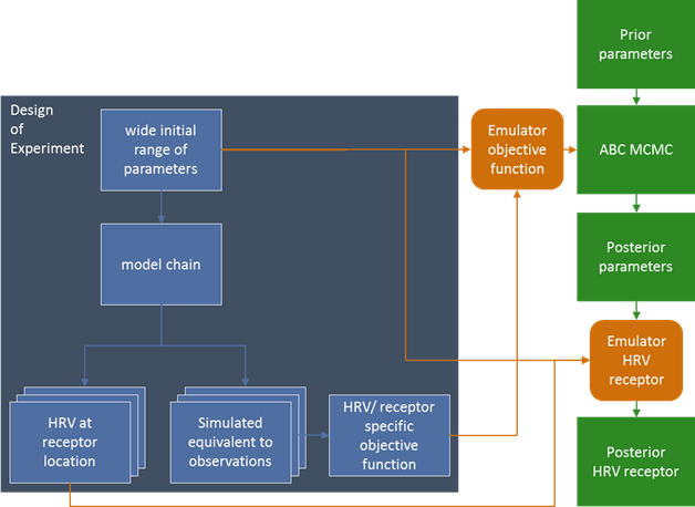
Figure 13 Uncertainty analysis workflow

HRV = hydrological response variable; ABC MCMC = Approximate Bayesian Computation Markov Chain Monte Carlo

In the design of experiment, a large number of parameter combinations are generated for the complete model sequence. The number of the parameter combinations is primarily determined by the number of model evaluations that can be afforded within the computational budget for that subregion. The parameters are generated through a Latin Hypercube sampling (Helton and Davis, 2003) that optimises the coverage of the parameter space. This results in a quasi-random but uniform sample across the range of each parameter. The ranges of parameters are chosen such that they are wide enough to encompass the prior parameter distributions, but sufficiently narrow to avoid numerical instability due to unrealistic parameter values. The ranges are defined based on the results of a stress test and the experience of the model team. A stress test consists of running the model a limited number of times with extreme parameter combinations. If the model proves to be stable for these extreme parameter combinations and provides results consistent with the conceptualisation, it inspires confidence that the model can be successfully evaluated for the parameter combinations of the design of experiment. The stress test also serves as a tool to identify and remediate any errors or inconsistencies in the implementation of the conceptual model in the numerical model.

The chain of numerical models generates the quantity of interest, the hydrological response variable, at a predefined set of points in space and time. These points in space can be used to directly assess potential changes or impacts, or they can provide the basis for an interpolation that may be able to assess potential impacts. In addition to those predictions, the model outputs corresponding to observations are stored as well. For a groundwater model this can be the simulated value of groundwater level at the time and place a head observation is available. A single model sequence run will result in multiple hydrological response variables at several locations and times in the subregion or bioregion.

The most computationally intensive step in the workflow is evaluating the original model sequence for all parameter combinations. This results in a dataset of parameter combinations and their corresponding simulated equivalents to observations and the predictions. For each prediction an emulator will be trained with the design of experiment results. The emulator chosen is a local Gaussian process approximation (laGP) (Gramacy, 2013; Gramacy and Apley, 2015).

Observations are not emulated directly. The observations are combined in a summary statistic for the Approximate Bayesian Computation process and the summary statistic is emulated.

In Approximate Bayesian Computation a summary statistic is defined to assess the quality of the model, together with an acceptance threshold for this statistic. During the Monte Carlo sampling of the prior parameter distributions, only parameter combinations that meet the acceptance threshold are accepted into the posterior parameter distributions. The Approximate Bayesian Computation methodology allows the tailoring of the summary statistic to individual predictions. For example, to predict change in annual flow, the summary statistic only contains the observations of annual flow. For a groundwater level prediction, the summary statistic can be a weighted sum of the head observations in that aquifer, with higher weights for observations close to the prediction location, together with constraints on the overall model balance. This type of summary statistic optimises the use of local information, while ensuring the overall water balance is respected.

For each prediction a tailored summary statistic is defined and the Approximate Bayesian Computation Monte Carlo sampling is carried out until the posterior parameter distribution has a predefined large number of samples. These posterior parameter distributions are evaluated with the emulator for the prediction to arrive at the posterior predictive probability distribution.

As there is no guarantee that for each prediction an emulator can be created that will adequately capture the relationship between the model parameters and the predictions, each emulator is systematically tested using cross-validation. Emulators that do not satisfy predefined performance criteria are not used in the analysis. For these predictions, the predictive posterior probability distribution cannot be obtained and only the median of the design of experiment runs is reported.