5.2 Design construction

The selection of design points (or scenarios) for consideration by the experts occurs prior to the receptor impact modelling workshop in two stages. First, potential candidate design points are identified. This stage uses hydrological model output and hydrology expertise to identify plausible bounds on the relevant hydrological response variables. Second, design points are selected from the set of candidate points in such a way to optimise the design subject to the structure of the design matrix as described above.

5.2.1 Candidate point selection

The number of samples is set equal to the total number of parameters in the full model that describes the quadratic surface, which fully interacts with the reference period and future period, along with the parameters that correspond to the intercept, the long-term assessment year and the influence of the receptor impact variable from the reference assessment year.

For unconstrained designs, the candidate design points are defined by a factorial design with corner points determined by the ranges of the hydrological response variables in the reference period. The centre values are typically set to the mid-point of the hydrological response variable ranges for each marginal (Figure 13, top) but occasionally modified, for example, to the logarithmic scale. In the future period, the candidate points are similarly drawn from a factorial design for the hydrological response variables in the future period augmented by low and high values for the terms: future period, long-term assessment year in the future period and ; this results in a factorial design used to generate the candidate set in the future period.

The case of constrained or restricted design regions is considered in Section 5.2.3.

5.2.2 Design point selection

The -criterion (Chaloner and Verdinelli, 1995) seeks to maximise the objective function:

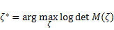
where 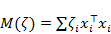, with the notation that is a row vector of , and where is a probability measure on the design region with , where is the number of samples at the th design point and with the total number of samples. The numerical solution uses the optimisation algorithm of Federov (1972) as implemented by Wheeler (2004) and Wheeler (2014) separately applied to the candidate design points generated for the reference and future assessment years. The resulting optimised solutions are randomly ordered within each assessment year. In all cases, the elicitation procedure begins with elicitations in the reference year before progressing to the short-term assessment year and finishing with elicitation in the long-term assessment year (Figure 12).

Figure 13 Constraints and design point selection for simplified surface water configurations considered only within the reference period

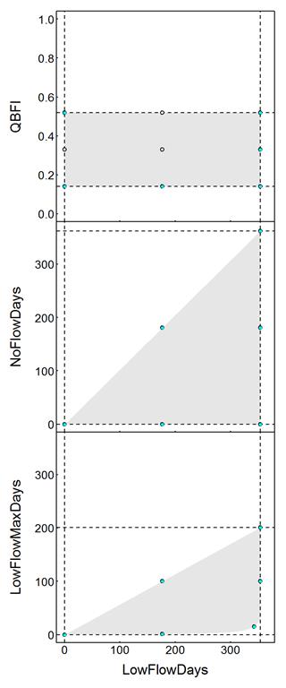
The average number of low-flow days over a 30-year period is given on the x-axis. Top: QBFI, an index of the ratio of surface flow to baseflow, ranges between 0 and 1. The ranges estimated from the stochastic hydrology modelling output are given by black dashed lines. The resulting feasible design region is the shaded area. Candidate design points generated from the 3 by 3 factorial design given by the design region ranges and mid-points are shown by open circles. The cyan points are those selected by the D-criterion optimisation algorithm. Middle: NoFlowDays is similarly defined as LowFlowDays but uses a more extreme flow threshold. NoFlowDays cannot be greater than LowFlowDays, which produces the constrained design region (shaded area). Bottom: LowFlowMaxDays is the maximum duration of low-flow events. The defined relationships between these hydrological response variables result in a complicated set of constraints. The candidate design points affected by the lower bound were adjusted and the revised design points are shown for this example.

5.2.3 Restricted design regions

There are two general strategies to deal with constrained design regions. The first approach would be to propose a set of candidate design points for the unconstrained design region, then optimise the selection of candidate design points from the subset that meet the constraints. The second approach would be to modify the candidate points so as to meet the constraints before optimising the set of design points.

For some elicitations, the first approach is sufficient. For example, in the Gloucester subregion ‘Perennial – gravel/cobble streams’ landscape class percent canopy cover receptor impact model, EventsR0.3 and EventsR3.0, respectively, serve as proxies for overbench and overbank flood events. The number of overbank flood events (EventsR3.0) cannot be greater than the number of overbench flood events (EventsR0.3). Another example is the relationship between the number of no-flow days (equivalently, zero-flow days) and the number of low-flow days. A no-flow day is a day when the flow does not exceed a negligible value, whereas a low-flow day occurs if the daily flow does not exceed a higher value that corresponds to a defined level of low flow. The number of no-flow days therefore cannot exceed the number of low-flow days. This latter example is shown in Figure 13 (middle) for the reference period.

For more restrictive constraint relationships, the simple lattice structure approach to generating candidate points may lose too many candidate points once the constraints are applied. However, in such cases for the receptor impact models considered here, a small adjustment may be applied that brings some of these excluded lattice points back into the feasible design region. The D-optimality algorithm can then be applied to these adjusted candidate points. An example is given below.

This second approach is necessary for combinations of hydrological response variables composed of average number of days of low flow and the average maximum duration of the event, defined as the number of contiguous days separated by a full day over the low-flow threshold. The definitions for these two hydrological response variables impose a complicated set of constraints. The maximum duration of low-flow events within a year, given by , must be less than the number of total low-flow days (), but not below the curve given by , thus, . Let the coordinates of a non-compliant candidate point drawn from the factorial lattice be given by , where 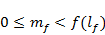. The distance from this point to an arbitrary point is given by:

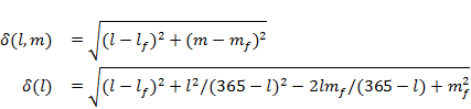
where the second line gives the distance to an arbitrary point on the curve that is obtained by substituting into the first line. Differentiating this result gives:

Setting gives the quartic polynomial equation:

The derivative is positive for . The curve is therefore monotonically increasing within the feasible region and a single real root satisfies the constraints, 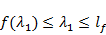. Thus, the solution for the sought-after feasible candidate point is given by the coordinates, . A graphical example is given in Figure 13 (bottom). For example, the candidate point in the lower right corner has been visibly adjusted inward to the closest point within the feasible design region.