5.1 The general statistical model

The receptor impact model framework specifies a statistical model for the response function parameterised by expert opinion (Hosack et al., 2016, 2017). A modelling approach is adopted that allows for different types of empirical data, , such as abundance, density, quadrat counts or presence–absence using generalised linear models (McCullagh and Nelder, 1989). The observation model for data , , is assumed to be from the exponential family and is conditioned on the expected response, , with possibly additional parameters that pertain only to the observation model. This expected response is mapped to the linear predictor, , by an invertible link function, . The linear predictor depends on the design point defined by the vector of known covariate values and the vector of unknown coefficients through the linear function:

The above assumptions lead to the construction of a prior for the unknown parameters with a generalised linear model with defined observation model, link function and design point .

5.1.1 Choice of link function and observation models

The generalised linear model allows for a wide variety of potentially observable responses that can be identified within a receptor impact model. Many options of link function and observation model will be available for a given receptor impact model. Guidance is provided here to assist this important selection process. The elicitation approach assumes that counts over the non-negative integers follow a Poisson distribution (with unknown varying intensity) and counts from a finite sample size follow a binomial distribution (with unknown varying probability); these are standard choices from the exponential family for count data. For the Poisson case, two link functions will be required (log and complementary log-log, ‘cloglog’), complicating the model fitting. For the binomial case, only the cloglog is required (with and without an offset). For both cases the above approach can be accommodated by the currently available methods for eliciting subjective probability distributions. These choices establish a correspondence among non-negative counts, bounded non-negative counts and presence–absence receptor impact variable models. Although the below choices develop log link models for discrete observations , note that the analogue for non-negative continuous data is given by the Gaussian observation model coupled with log link.

5.1.1.1 Poisson

Let 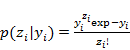with 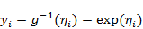with mean given by the inverse of the canonical log link function of the linear predictor 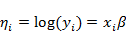with known covariates and unknown parameters . The intensity of the inhomogeneous Poisson process is given by .

5.1.1.1.1 Support

The support of is over the non-negative integers, . For example, it is applicable to a setting with a countable number of individuals in a given area.

5.1.1.1.2 Elicitation target

The expected value of the response is the average number of individuals in a given area over a specified time period.

5.1.1.1.3 Probability of presence

The probability of observing a zero count is 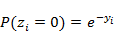. Let equal the probability of presence:

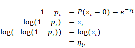
where the function is called the complementary log log function (cloglog). Therefore, eliciting the probability of presence given the complementary log log link function is a replacement for eliciting the expected abundance, when the expected abundance is very low (near zero). If the expected abundance is far from zero, then the probability of presence is effectively 1 and so will not provide much information on . It is then better to stick to the log link and target the magnitude (e.g. abundance).

5.1.1.2 Binomial

Let with mean given by the inverse complementary log log link function and linear predictor . The expected proportion of presences (successes) is given by .

5.1.1.2.1 Support

The support of is over the bounded non-negative integers, . For example, it is applicable to a setting with the number of observed presences given a total number of observations in a given area or transect.

5.1.1.2.2 Elicitation target

The expected value of the response is the expected proportion of presences given the observations

5.1.1.2.3 Probability of presence

The probability of observing a zero count is 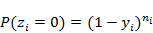. Let equal the probability of presence:

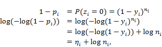
where is an offset. The left-hand side on the second line in Equation (18) is again the complementary log log link function, which is also the assumed link function for this binomial generalised linear model. Therefore, the probability of presence given the complementary log log link function is equivalent to eliciting the expected proportion of presences with an offset.

5.1.2 Structure of design matrix

The elicitation of for the short- and long-term future periods depend on the hydrological response variables and a realised value of . The model formulation uses a quadratic surface to describe the relationship between hydrological response variables and receptor impact variables. The curvature allowed for the fact that most ecological variables will have optimal values at intermediate levels of an environmental gradient. For example, not enough water can lead to tree mortality due to drought, whereas too much water can lead to tree mortality due to flooded conditions.

A fundamental issue in developing the receptor impact models is that for a significant number of variables their current state across the landscape class is unknown, which obviously impacts on the ability to make predictions. A key example is groundwater depth. Change in depth can be modelled but there will not be detailed maps of groundwater depth across all subregions or bioregions. Another example is information on the presence, absence or condition of an ecological community. This data will typically be incomplete or missing entirely. Given these constraints, models will sometimes need to accept covariates defined in terms of deviations in hydrological response variables relative to ‘reference’ conditions.

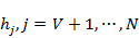
The model structure is determined by the design matrix that is composed of the design points For hydrological response variables that vary in both the reference and future periods, the functional form is a second order polynomial on the linear predictor that allows interactions among hydrological response variables, the reference period and the future period (Equation 19). For hydrological response variables that are defined relative to the reference period, the values of the hydrological response variables are fixed by definition in the reference period. For a given receptor impact model, enumerate the hydrological response variables with varying values in the reference period by , and the hydrological response variables without varying values in the reference period by :

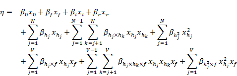
The coefficients are defined in Table 3.

Table 3 The coefficient notation, attributed names and corresponding covariates as defined by the structure of the design matrix for the full model

HRV = hydrological response variable, RIV = receptor impact variable

5.1.2.1 Influence of the receptor impact variable from the reference assessment year

Note that by construction the covariate named with the symbolic shorthand as in Table 3, which has zero values in the reference period, can be interpreted as an interaction between and the future period binary factor, . To see the ecological interpretation of in the above equation for that is associated with the covariate (Table 3), which is equivalent to the entrywise product between and , first consider a model developed for the unknown quantity , with a known offset,

where the term:

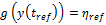
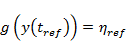
captures the hydrological response variable effects on the receptor impact variable. The offset is specified as the function:

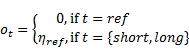
with the value of in the last line assumed known. Given this specification of the offset, the unknown quantity is defined by:

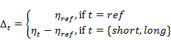
again, with the value of in the last line assumed known.

In the above model for , the term measures the association between the receptor impact variable and the future change in on the linear predictor scale, and so it includes an interaction with the binary covariate such that this term has no influence on the receptor impact variable in the reference period. The coefficient therefore defines the relationship between and the future change when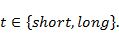

The above model for can be rewritten with the known offset moved to the right-hand side:

Consider this model applied to a scenario in the reference period:

where the known offset is set to zero when , so that 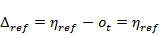. The unknown only appears on the left-hand side, as desired (it is the response variable). For a scenario in the future period with 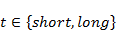, the model instead takes the form:

where 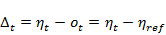with known value of for 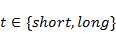. It can be seen that 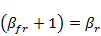for a future scenario. The coefficient associated with the covariate in the original model for above provides the relationship between and the future when

All parameters thus have an ecological interpretation. Importantly, dependence of the receptor impact variable on the hydrological response variables is modelled jointly across both reference and future scenarios. Moreover, all unknown parameters appear linearly in the above equations. This linear property will be used by the method of estimation for the unknown parameters described in Chapter 7 . For estimation, the choices for the values of in the known offset function are derived from the elicitation scenarios as described in Chapter 7. Future predictions for will depend on known generated in the reference assessment year as described in Chapter 8. Example receptor impact models with specified design matrices are given in Section 5.3.