8.2 Monte Carlo approximation

The realisations of the unknown coefficients are independent of the hydrological response variables (Figure 14). In particular, the realisations of are independent across the assessment units. Spatial dependence may nevertheless be introduced into the receptor impact variable predictions across assessment units to the extent that spatial dependence is captured by the hydrological response variables.

Monte Carlo approximations to the above joint distributions are available through the method of composition (Tanner, 1996). To sample from 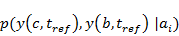(Equation 41):

Repeat the above steps times to obtain simulations and store all values. Samples from the marginal 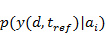are obtained by considering only the simulations .

Next, to sample from :

Repeat times.

Similarly, to sample from :

Repeat times for each assessment unit .

Given the simulated values of the jointly dependent receptor impact variable , Monte Carlo approximations of any function of , are also available. For example, simulated values of the actual change and relative change for the short-term assessment year are given by:

and likewise for the long-term assessment year, Predictions are thus available for all assessment units.

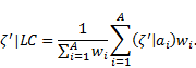
Aggregated predictions to the landscape class are also available with simulated values of the landscape class level weighted averages. Given simulated values of a quantity for each assessment unit, such as a prediction of the receptor impact variable or some other function such as the actual or relative change, the landscape class prediction is given by:

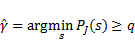
For each landscape class and for each assessment unit, a set of quantiles, which includes the 5th, 10th, 15th, 20th, 25th, 30th, 35th, 40th, 45th, 50th, 55th, 60th, 65th, 70th, 75th, 80th, 85th, 90th, and 95th quantiles, was estimated through the above Monte Carlo approach for each unknown quantity of interest that depends on the receptor impact variable. Let be the inverse cumulative distribution function for . The qth quantile is given by, for . Let the empirical cumulative distribution function of the samples of be given by . A Monte Carlo estimate of the qth quantile is then given by:

Extreme quantiles are more sensitive to approximation error by the Monte Carlo method, and larger sample sizes reduce Monte Carlo error. The number of receptor impact variable simulations can be made arbitrarily large. However, the composition sampling that preserves the joint dependence between the receptor impact variables and the hydrological response variables is limited by the number of realisations available from the hydrological modelling simulations.

Rather than quantiles, it may also be of interest to report the average of the above unknown quantities either at the level of assessment units or landscape class or both. A mean estimate for an unknown quantity is trivially obtained by taking the sample mean of the above Monte Carlo simulations.