3.1 Considerations in streamflow modelling
Streamflow modelling (also called rainfall-runoff modelling) takes input from meteorological data (primarily rainfall and potential evaporation) and produces inflows to the stream network. Almost all streamflow models contain parameters with unknown values, which must be estimated by calibration. This calibration is usually done by comparing predicted streamflows with those observed at streamflow gauging stations (Viney et al., 2014).
The major challenge in streamflow modelling is to produce credible predictions of streamflow in ungauged parts of the modelling domain. This usually involves the estimation of appropriate model parameters to use in those parts of the landscape. This process of parameter estimation in the absence of direct calibration is called regionalisation (Viney et al., 2014).
There are two broad categories of regionalisation. One involves using parameter values from a gauged catchment that is considered to share similar characteristics (climate, soils, vegetation, geomorphology) to the ungauged area. Often, it is found that the simple expedient of using parameters from the nearest gauged catchment is among the best regionalisation methods. Implicit in this nearest-neighbour approach is the assumption that catchments in proximity are likely to share similar physical and hydrological characteristics and that therefore, optimal models of each of them will also share similar parameter values. However, there is a significant degradation in model performance with this type of regionalisation as regionalisation distance increases (Viney et al., 2014).
The second regionalisation approach involves simultaneous calibration of a model using observations from several nearby gauging stations. In this approach, the calibration procedure uses a single objective function that combines the prediction responses in all gauged catchments and results in a single set of model parameter values that provide best fit to the streamflow observations from all gauges. The key assumption here is that if a single set of parameter values provides good predictions in the gauged catchments it might also be expected to provide good predictions in adjacent ungauged areas. This regionalisation approach is called regional calibration (Viney et al., 2014). Unlike nearest-neighbour calibration, the performance of regionally calibrated models does not degrade with distance from the calibration catchments and is likely to lead to more stable predictions in ungauged parts of the modelling domain.
The temporal and spatial scales of streamflow modelling are dictated largely by the temporal and spatial scales of the available meteorological input data. The bioregional assessments (BAs) use meteorological data from the dataset of the Bureau of Meteorology’s Australian Water Availability Project (Bureau of Meteorology, 2016a). These data use a daily time step and are presented on a grid with spacing of 0.05 degrees of latitude and longitude (approximately 5 km). Thus, it follows that the smallest temporal element in the raw streamflow modelling is one day and the smallest spatial element is 0.05 degrees. Note that this raw spatial scale does not preclude modelling at finer spatial scales through interpolation, and nor does it preclude the assessment of the impacts of coal resource developments with sub-pixel extents.
3.2 Modelling options
A large number of streamflow models exist in the literature and many of them have been applied widely in Australia. These include:
- GR4J (Perrin et al., 2003)
- Sacramento (Burnash et al., 1973)
- Simhyd (Chiew et al., 2002)
- IHACRES (Croke et al., 2006)
- SMAR-G (Goswami et al., 2002)
- AWBM (Boughton, 2004)
- AWRA-L (Viney et al., 2015)
- LASCAM (Sivapalan et al., 2002).
The first six of these models are typical rainfall-runoff models. Most are relatively parsimonious in their parameterisation. They are amenable to both nearest-neighbour regionalisation and regional calibration. Studies comparing their prediction quality in Australia (e.g. Viney et al., 2014) generally indicate that these models have relatively similar prediction performances. Sacramento is the model usually adopted to provide tributary inflows in state agency river system models (e.g. IQQM and Source Rivers; see Chapter 4).
AWRA-L (Viney et al., 2015) is designed for use in a regional calibration setting using gridded input. This regional calibration approach is assisted by the model’s explicit inclusion of vegetation density as a factor controlling streamflow generation. AWRA-L is typically calibrated Australia-wide to yield a single continental parameter set. A recent comparison study by Viney et al. (2014) shows that AWRA-L provides streamflow predictions with an improved fit to observations relative to the Sacramento and GR4J models whether the latter are implemented using either nearest-neighbour regionalisation or regional calibration. AWRA-L is part of a suite of models in the AWRA (Australian Water Resources Assessment) system (Bureau of Meteorology, 2016b) which also includes a river routing module (AWRA-R). At present, these two components operate together in an uncoupled fashion, but work is underway in CSIRO to develop a fully coupled AWRA model. This fully coupled model is not available for use in the current round of BAs, but may be available for future BAs.
LASCAM has been designed for use at the large catchment scale. Like AWRA-L, LASCAM explicitly includes the effects of vegetation density and has been designed for use in a regionally-calibrated context. LASCAM also includes an embedded routing scheme, thus meaning that it can also replicate many of the functions of a river system model. LASCAM has recently been used in a study in the Namoi subregion by Schlumberger Water Services (2012), but has not been applied in any of the other subregions. This application in the Namoi subregion appears to have been done with limited calibration. Unlike the other candidate models, LASCAM has not yet been implemented using gridded input, although this could be readily done. It also requires more input data and can be difficult and time-consuming to calibrate properly.
3.3 Recommended modelling approach
It is desirable – although by no means requisite – that a consistent modelling approach be adopted across all the bioregions in the Bioregional Assessment Programme. Since the adopted model will be used for both futures (baseline and coal resource development pathway (CRDP)), it is also desirable that a common set of model parameters be used in each subregion or at least in each major river basin in a subregion. This is not just for practical reasons, but also to ensure that the true spatial heterogeneity of runoff generation is represented across the modelling domain, with no significant spatial discontinuities that might arise as artefacts of regionalisation. This rules out the use of nearest-neighbour regionalisation, although all candidate models are capable of being deployed in a regional calibration mode.
Given its adoption for the Bureau of Meteorology’s water accounts and assessments (Bureau of Meteorology, 2016b), its prediction performance relative to other rainfall-runoff models, its ready availability to the BA modelling team, and the ability to make the code and executables publicly available, it is recommended that AWRA‑L be the streamflow model adopted for BAs. Furthermore, it is recommended that AWRA-L be implemented using regional calibration.
In the main – and modelling of impacts of coal resource development notwithstanding – this approach falls somewhere between the adopt and adapt strategies canvassed in Section 2.2.
There is a requirement that the models used in the BAs, including their code, executables, data and parameters, be made publicly available. All open access data used in the AWRA-L model will be made available through data.gov.au as well as all output data from the model. The metadata for the model will direct users to where the model can be downloaded.
3.4 Streamflow modelling methodology
3.4.1 Spatial and temporal resolution
AWRA-L operates on a daily time step using gridded input. It is applied in a modelling domain that includes not just the subregion itself, but also extends upstream of the subregion boundaries to include all upstream tributaries, and downstream of the subregion boundaries to include all of the preliminary assessment extent and all of its tributaries. Raw output is gridded at the same spatial scale as the input data.
Each spatial unit (grid cell) in AWRA-L is divided into a number of hydrological response units (HRUs) representing different landscape components. Hydrological processes are modelled separately for each HRU before the resulting fluxes are combined to give cell outputs. The current version of AWRA-L includes two HRUs which notionally represent (i) tall, deep-rooted vegetation (i.e. forest), and (ii) short, shallow-rooted vegetation (i.e. non-forest). Hydrologically, these two HRUs differ in their aerodynamic control of evaporation, in their interception capacities and in their degree of access to different soil layers.
3.4.2 Data requirements
AWRA‑L requires the following data:
- gridded daily rainfall
- gridded daily potential evaporation (or the raw data from which to estimate it – e.g. gridded daily maximum and minimum temperature, vapour pressure, wind speed, etc.)
- proportion of deep-rooted vegetation in each grid cell
- time series of remotely sensed leaf area index for each grid cell
- daily streamflow at multiple sites
- catchment boundaries for each streamflow measurement site.
The meteorological and vegetation datasets are readily available to modellers in the Bioregional Assessment Programme and are ready to use immediately. Streamflow records are available from the Bureau of Meteorology. However, there are substantial variations in the quality of observed streamflow records (Zhang et al., 2013), so there is likely to be a role for programme staff to vet data from individual streamflow gauges before it can be used in model calibration. Catchment boundaries can be extracted from the Australian Hydrological Geospatial Fabric (Geofabric) dataset (Bureau of Meteorology, 2016c) using the best available digital elevation and gauge location information.
3.4.3 Calibration
Because of the nature of the BA application – in particular that it is mostly focused on the differences between model runs, rather than on absolute predictions, and that its results are presented in an uncertainty framework – the importance of model calibration is less than it is in most other surface water modelling applications. Nonetheless, model calibration still forms part of the methodology.
The streamflow model is calibrated separately in each subregion using streamflow observations from gauging sites in and near the subregion. Selection criteria for calibration gauges include that the gauges, where possible, should:
- have catchment areas greater than 50 km2
- have at least ten years of observed streamflow data since 1983
- have no significant flow regulation (e.g. upstream reservoirs, irrigation withdrawals, mining)
- be non-nested (i.e. not directly upstream or downstream of another selected gauge).
Since the objective of this calibration is to obtain a single set of model parameters, there should be no impediment to using nearby observations even if they are from catchments outside the modelling domain. Indeed, some subregions contain few, if any, streamflow gauges, so it is necessary to use data from further afield or to relax one or more of the selection criteria. Observations from at least two gauges, and preferably more, should be used in the calibration process. The prediction performance in these calibration catchments should be summarised statistically and combined into a single objective function for optimisation.
In most subregions, the parameters to be calibrated are those designated by Viney et al. (2015) as the parameters that are typically and routinely calibrated in AWRA-L applications.
Two calibration runs are performed, one with an objective function biased towards high flows and one with an objective function biased towards low flows. This is because streamflow at both ends of the hydrograph spectrum are likely to be important for receptor impact modelling and for water balance estimation.
The objective functions used in calibration should seek to optimise the joint prediction of temporal variability in the streamflow hydrographs and the overall bias in model prediction. This can be achieved by basing calibration on the methodology of Viney et al. (2009). In the case of the high flow calibration, a function F, which characterises prediction quality, is evaluated for each catchment. This function is given by:
|
|
(1) |
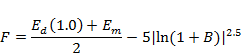
where Ed(1.0) is the daily Nash-Sutcliffe efficiency with a Box-Cox lambda value of 1.0, Em is the monthly Nash-Sutcliffe efficiency and B is the bias (prediction error divided by sum of observations). The optimiser then maximises an objective function that is given by:
|
|
(2) |
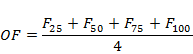
where Fn is the nth percentile of the F values in the calibration catchments.
In the case of the low flow calibration, F is given by:
|
|
(3) |
where Ed(0.1) is the Nash-Sutcliffe efficiency with a Box-Cox lambda value of 0.1. These F values are used along with the same functional form for the objective function as for the high flow calibration.
Although the two resulting deterministic model predictions are not used directly in reporting BA outcomes, they are used in BAs to:
- inform prior parameter distributions for the uncertainty analysis
- provide recharge estimates for surface water – groundwater modelling
- populate water balance estimation.
The calibration period used will depend in part on the temporal coverage of the available streamflow observations. Ideally, the calibration period should cover at least 20 years – preferably in recent decades – and should be preceded by at least 10 years of spin-up to allow water stores to equilibrate. In subregions or river basins where 20 years of observational data are not available, consideration should be given to including streamflow observations from farther afield into the response dataset.
Previous applications and assessments of AWRA‑L (Viney et al., 2014) have indicated that there is little difference in model performance between the catchments used in calibration and those used in independent validation. For this reason, it is recommended that no independent validation be done on AWRA‑L modelling in the Bioregional Assessment Programme. This frees up all the available streamflow data to be used in calibration to better constrain model parameters. It also means that the quality of the model’s performance in the calibration catchments will provide a strong indication of its performance in other parts of the modelling domain. There will, however, be validation of model performance during the uncertainty analysis against observations of several metrics of streamflow.
3.4.4 Modelling impacts of coal resource development
Coal resource development is defined with two potential futures:
- baseline coal resource development (baseline), a future that includes all coal mines and coal seam gas (CSG) fields that are commercially producing as of December 2012
- coal resource development pathway (CRDP), a future that includes all coal mines and coal seam gas (CSG) fields that are in the baseline as well as those that are expected to begin commercial production after December 2012.
The difference in development between CRDP and baseline is defined as the additional coal resource development, all coal mines and coal seam gas (CSG) fields, including expansions of baseline operations, that are expected to begin commercial production after December 2012.
Highlighting the potential impacts due to the additional coal resource development, and the comparison of these futures, is the fundamental focus of a BA.
In order to assess the impacts due to the additional coal resource development, the surface water modelling undertaken in the BAs must produce and compare outputs from two simulations: a baseline simulation without the additional coal resource development and a CRDP simulation with the additional coal resource development.
The starting date for the two simulations is January 2013.
Any pre-existing coal resource developments (i.e. those that were commercially producing before 2013) are included in both simulations. The modelling outputs report the changes in surface water availability between the baseline and CRDP.
Some proposals for coal resource developments contain insufficient information to allow meaningful modelling. For example, they may be lacking in groundwater pumping rate information or detailed development footprint information. Such proposals will be dealt with through commentary only. Only those proposals that do have sufficient information will be modelled and it is those developments that are considered here and are of relevance to the modelling outcomes in product 2.5 (water balance assessment) and product 2.6.1 (surface water numerical modelling).
3.4.5 Climate input
The key outcome of the BAs is in determining how the additional coal resource development leads to changes in flow regime and risks to water-dependent assets. In reality, this can be achieved using any (consistent) climate input signal for the two simulation runs. Nonetheless, it is possible that the magnitudes of these changes could be different when the coal resource developments are superimposed over different baseline climates. It is therefore ideal – though not crucial – that the projections into the future for both simulations use climate input that reflects likely climate change trends. To be consistent with the philosophy of the CRDP, a single ‘mid-range’ future climate time series will be constructed.
It is important to recognise that the BA is not a climate change study. The main focus is on the impacts of coal resource development activities on water resources and water-dependent assets. Both the baseline and CRDP simulations will use the same climate input; BA is interested in the differences between the two simulations caused by the coal resource development, not the impact of climate change on streamflow characteristics.
3.4.5.1 Construction of future climate input
As the future climate is unlikely to be stationary, it is desirable to incorporate a trajectory of likely climate change in the future climate time series from January 2013 to December 2102. To avoid a climate change signal being present in the donor time series used for creating a future climate time series, and to ensure the donor series has the highest notional data quality, a shorter 30-year period will be used as the basis for generating the future climate time series. A recent 30-year period (January 1983 to December 2012) will be assumed short enough that a changing climate trend is not significant and assumed to be long enough to be representative of the climate variability (i.e. contains the millennium drought in southern Australia and the floods of 2011 in some subregions). The 30-year historical climate time series will be repeated three times to create a 90-year time series.
Global climate model (GCM) outputs will be downscaled separately for each 30-year period using the ‘seasonal scaling’ approach described by Chiew et al. (2009). This is neither the most sophisticated nor the simplest method of downscaling, but has been proven to be effective and the method will require little development to be adapted for use in BA. The three 30-year periods will be modelled as step changes in climate, nominally representing 2030, 2060 and 2090. The seasonal scaling method modifies the historical time series using seasonal scaling factors and then modifies the daily rainfall according to the projected change in temperature and the GCM-predicted change in rainfall per degree of climate change.
The very simplistic representation of the future climate time series and ignoring of the uncertainty in the future climate are justified as the BA projects are not investigating the impact of climate change upon the assets and receptors. The only two forward modelling runs that will be conducted are the baseline and the CRDP. The future climate time series will be used for both runs and so it will not be possible to disentangle the impact of the future climate from the impact of the future coal resource development upon the assets and receptors.
The landscape modelling will be conducted using the 90-year future climate time series on a daily basis to create the input time series for the river and groundwater modelling (runoff and recharge, respectively). The river modelling will be conducted using the entire 90-year future climate time series. The groundwater modelling will be conducted on a monthly time step for the 90-year period until 2102 to enable the surface water – groundwater interactions to be accounted for in the river modelling.
3.4.5.2 Choice of climate change signal
In each subregion, the future climate series will be based on the projections of a single global climate model (GCM) and a single emissions scenario. This choice of GCM and emissions scenario must be transparent and defensible. There is considerable uncertainty in future climate projections so a desktop study will be conducted of previous comparison studies to determine an appropriate GCM for each subregion.
In all bioregions, climate projections from 15 GCMs[1] are available. Associated with each GCM are local scaling factors which give the change in rainfall expected per degree of global warming. We will use scaling factors for the AR4 emissions scenario A1B (IPCC, 2007). Depending on GCM, the scaling factors may be seasonal or monthly. Together with seasonal or monthly trends in historical rainfall, it is possible to use these scaling factors to assess the change in mean annual rainfall associated with each GCM. In each subregion, we will choose the scaling factors from the GCM that produces the median change in mean annual rainfall.
3.4.6 Methodological variations among the bioregions
It is expected that in all subregions where new modelling is being undertaken, the application of the landscape model will closely follow the methodology outlined in Section 3.4.
The most likely scope for variation is in the selection of a suitable objective function for calibration of the low flow parameter set. This choice might be dictated at the local level by two factors: the nature of the flow characteristics and the required hydrological response variables. An objective function for a low flow calibration, for example, might include a metric describing the degree of intermittency in streamflows. Such a metric, however, might be redundant in a subregion where streams are typically permanent.
In subregions where analysis will be based on existing model results – which are likely to come from models other than AWRA-L – it is likely that these results will have been generated from a single set of model parameters, most likely one that is predicated largely on high flows. This means that projected impacts on low flow characteristics may be more uncertain in these subregions.
