
6.2.1 Structure of elicitation
The target of the elicitation is the unknown value of the receptor impact variable,  . The receptor impact variable is defined such that it has a direct interpretation relative to potential observables and expert knowledge (Chapter 4). For example, in a Bernoulli response model considered at the ith hydrological scenario, a (hypothetical) observation
  , corresponds to either a presence or absence, and
  is interpreted as the probability of presence. In a Poisson response model where corresponds to a count,
  is interpreted as an intensity that may relate to the annual average abundance over a defined spatial scope. The experts provide subjective probability distributions describing the receptor impact variable estimates conditional on a hydrological scenario summarised within the design point
  (see Section 5.2.2). The elicited subjective probability distributions are assumed independent conditional on the hydrological scenarios.
6.2.2 Elicitation of subjective conditional probabilities
Conditional on the design point  , the goal is to elicit a normal distribution for
  with the mean and variance parameters summarised into the parameter vector
  . An elicitation of fractiles (equivalently, percentiles or quantiles) for the target
  , given the monotonic link function, directly translates into fractiles for the conditional normal distribution of the linear predictor,
  . The experts are asked for each design point to perform judgements of equal odds in three steps:
- What value do you believe gives a
 chance that the true receptor impact variable is lower? (This obtains a prediction of the median,
  )
) - Assume that the true value is really below . Given this information, what value do you believe gives a chance of being above or below the true value of the receptor impact variable? (This is the first quartile,
 )
) - Assume that the true value is really above . Given this information, what value do you believe gives a chance of being above or below the true value of the receptor impact variable? (This is the third quartile,
 ).
).
The parameters  are then chosen to minimise the information lost by approximating the elicited fractiles by a normal distribution. The elicited fractiles are assembled into the vector,
  where
where  . The extreme fractiles
  and
and  (possibly infinite) are determined by the support of . Let the probability intervals determined by these elicited fractiles be denoted by
  for
for  . Let
. Let  denote the histogram constructed by these elicited fractiles.
Fitted probability intervals for the approximating normal distribution are obtained by:
|
|
(31) |

where  is the subjective probability distribution function parametrised by .
The Kullback-Leibler divergence of  from the elicited , where subscripts denote dependence on and , is approximated by:
|
|
(32) |

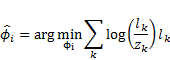
where is absolutely continuous with . The parameters are chosen so as to minimise the approximate Kullback-Leibler divergence of from :
|
|
(33) |
For each scenario, the values of the design point are portrayed and the group discusses the potential ecological response. The goal is to develop a probability distribution that is an acceptable representation of the experts’ beliefs. Of course, with unlimited time resources a suite of distribution families could be presented for consideration by experts. Resources in BA are not unlimited, however, and for consistency and efficiency the parametric distribution considered by the experts is defined by the models specified and described in Section 5.1. The following steps are then performed by the experts:
- Initial fractile assessments are elicited using the quartile method. These are plotted graphically as vertical dashed lines. Note that more fractiles than free parameters are elicited in an approach that is referred to as ‘overfitting’ (O’Hagan et al., 2006), which will permit feedback between the model representation and the group’s final probabilistic statement as detailed in the following steps.
- The corresponding fitted fractiles and density curve from the fitted probability density function
 are plotted as three vertical blue dashed lines and blue curve, respectively. The overfitting approach uses the parametric model to average across multiple probability statements. The parametric model is unlikely to exactly match the elicited fractiles from Step 1, and so this process encourages the group to evaluate the parametric model with respect to their beliefs. If the values for the matching fractiles are not acceptable, then the group returns to Step 1 and adjusts the elicited fractiles. These two steps are repeated as often as necessary until the group accepts the parametric model quantiles as acceptable.
 - The extreme deciles from are plotted as dashed blue lines. The group considers these new predictions and returns to Step 1 if the predictions are unacceptable.
- The group is allowed to consider other fractiles or cumulative probabilities as predictions from the parametric model. The group returns to Step 1 if these predictions are unacceptable.
- After completing the above feedback steps, the group is allowed to accept the elicited subjective probability distribution as a reasonable assessment of the expert opinion.
This process thus elicits from the group a subjective probability distribution of ecological response given the covariate values that make up the defined scenario. Note that the elicitation focuses on the distribution, not the raw fractile assessments (e.g. Step 1 above). The raw fractiles are used by the experts as ‘parameters’ to iteratively build a probability distribution that is an acceptable representation of their beliefs. The probability predictions made by the elicited probability distribution provide the final products that are assessed by experts for either acceptance or rejection and further iteration until the experts accept the probability distribution as a reasonable model of their beliefs. This process is repeated for each design point.