3.1 Methods for qualitative mathematical modelling

The following section contains a brief overview of qualitative mathematical modelling based on the construction and analysis of sign-directed graphs (or signed digraphs) and also equivalent approaches using matrix algebra. The signed digraph models in this section are very simple models presented only for pedagogical purposes. Applied BA examples can be found in product 2.7 (receptor impact modelling) (Figure 3).

3.1.1 Signed digraph methods for qualitative mathematical modelling

3.1.1.1 System structure and signed digraphs

Qualitative mathematical modelling proceeds by first determining system structure, which is defined by the variables of the system and the relationships by which they are linked (Puccia and Levins, 1985). In biological systems, variables are typically interacting populations of different species, and their dynamics can be accounted for by generalised Lotka–Volterra equations, where each contributes towards the birth or death of another. Similarly, the dynamics of human social and economic systems can be described by the interactions of different sectors and entities of society that control flows of resources, goods and services.

The variables and relationships in a model system are portrayed by sign-directed graphs, or signed digraphs, where a link from one variable to another ending in an arrow () represents a positive direct effect, such as a rate of birth that is increased by consumption of prey, and a link ending in a filled circle () represents a negative direct effect, such as a rate of death due to predation. All possible ecological relationships can thus be described:

Self-effects are shown by links originating and ending in the same variable, and are typically negative, as in self-regulated variables, but can also be positive ( ), where variables are self-enhancing. Usually, relationships between species can be restricted to being linear (e.g. Lotka–Volterra predator–prey interactions), although non-linear relationships (e.g. Holling functional responses) can also be incorporated. Here, the sign of a relationship can change when the system passes a threshold. This then leads to construction and analysis of alternative model structures (Dambacher and Ramos-Jiliberto, 2007).

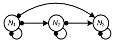
Once the structure of a system is defined, it is possible to analyse the system’s feedback which determines the qualitative conditions for system stability and perturbation response. These methods can proceed via analysis of the signed digraph through graphical algorithms or through equivalent algebraic analyses of the system’s community matrix. As an illustrative example, the Assessment team consider a signed digraph of a predator–prey community of size , where the top predator is an omnivore that feeds on the basal species (Figure 5):

Figure 5 A signed digraph of a predator–prey community of size n = 3, where the top predatorN3 is an omnivore that feeds on the two other prey species

3.1.1.2 System stability

The stability of a system can be judged and understood according to criteria that depend on the relative sign and balance of the system’s feedback cycles (Puccia and Levins, 1985; Levins, 1974, 1975, 1998; Dambacher et al., 2003b). In general, stability requires that the net feedback in a system is negative and that feedback at lower levels is stronger than feedback at higher levels in the system. Negative feedback ensures that a system’s dynamics are self damped, and stronger feedback at lower levels ensures that a system will not over correct and exhibit unrestrained oscillations. The conditions can be interpreted through specific algebraic arguments. In general, though, stability in this system depends on the relative weakness of feedback cycles involving omnivory. Here, the feedback cycle has the potential to destabilise the system through positive feedback, and the feedback cycle , even though it is negative in sign, has the potential to introduce excessive higher level feedback if it is too strong.

3.1.1.3 Perturbation response

The signed digraph (or its matrix equivalent) provides a mechanism to predict qualitatively how species abundance or biomass in the system as a whole change as a result of a sustained change to the rate of birth, death or migration in any one of the species (Puccia and Levins, 1985; Levins, 1974, 1975, 1998; Dambacher et al., 2002). As an example perturbation scenario, consider a positive input to , such as food supplementation that increases its rate of birth. The qualitative effect of this input to the other variables is determined by accounting for all of the feedback cycles of length that emanate from . This is accomplished by tracing all paths from the input variable to a responding variable and multiplying each path by its complementary subsystem, the resulting product is defined as a feedback cycle. The complementary subsystem is defined by the feedback of the variables not on the path from the input to the response variable. If the sign of this subsystem’s feedback is positive then it will switch the sign of the path to the response variable, otherwise the sign of the path will be unchanged. The signed digraphs below illustrate the formation of feedback cycles that are used to predict perturbation response. All links that enter the input variable and all links leaving the response variable have been removed; products of the remaining links then become the feedback cycles, which determine the sign of the response. For response of _, feedback cycles will be composed of the following links (Figure 6):

Figure 6 A signed digraph of a predator–prey community of size n = 3, showing a perturbation scenario where there is a positive input to N2

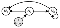
Here two feedback cycles determine the sign of the response of due to an input to . One feedback cycle, , is formed by a path which goes directly from to , and it has a complementary subsystem in the negative self-effect of . The other cycle, , is composed of a path with negative sign of length two. This path lacks a complementary subsystem, in which case the sign of the path remains negative. Since both feedback cycles are negative, the equilibrium abundance of is predicted to decrease as a result of supplementation of .

Next, consider the response of when there has been a negative input to , say through an increased rate of death, and note that for negative inputs the signs of the feedback cycles are switched. The sign of the response of is determined by the following links (Figure 7),

Figure 7 A signed digraph of a predator–prey community of size n = 3, showing a perturbation scenario where there is a negative input to N2

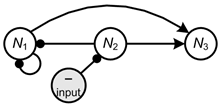
which form feedback cycles and . Here the response is ambiguous, as it is determined by feedback cycles of opposing sign.

3.1.1.4 Ambiguity and weighted predictions

The ambiguity in the response of can be resolved through consideration of symbolic inequalities. For instance, if it is believed that 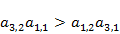, then the predicted response of will be negative. Dealing with ambiguity in this manner requires a knowledge of relative strength of interaction and an ability to make sense of contingencies presented by symbolic arguments. However, in larger systems, complex inequalities can arise, which are too difficult to interpret or comprehend. In these instances the Assessment team can employ a heuristic technique of weighting the net number of feedback cycles to the absolute number in a response (i.e. the weighted prediction for a response prediction is equal to the net number of feedback cycles divided by the total number of cycles (Dambacher et al., 2002)).

For instance, the predicted response of for an input to is completely ambiguous, as there is the same number of positive and negative feedback cycles. But if there were, say, a total of four feedback cycles in a perturbation response, three of which were positive and one negative, then the net number of cycles would be two and the weighted prediction of the response would be 2/4 = 0.5. The sign determinacy of responses with weighted predictions ≥0.5 has been shown to generally be greater than 90% through simulations using random parameter space (Dambacher et al., 2003a; Hosack et al., 2008); below this threshold the sign determinacy of responses declines to zero for weighted predictions equal to zero.

3.1.2 Matrix algebra methods for qualitative mathematical modelling

The preceding section presents an overview of qualitative modelling based on a general interpretation of signed digraphs, this section presents an equivalent analysis based on a system’s community matrix, as derived from a system of equations. Computer programs for these analyses can be found in the most recent revision of Supplement 1 of Dambacher et al. (2002).

Rates of growth for n interacting populations can be described by a system of linear equations:

where the per capita rate of change in population abundance of is controlled by density-independent rates of birth , death , immigration and emigration, and density-dependent interactions. Generally stated as:

the growth function of each population is determined by the system’s variables () and growth rate parameters 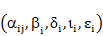; the latter can be collectively referred to as a vector p of length m. At equilibrium, population abundances (Ni^*) are unchanging and defined by:

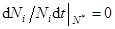
In the neighborhood of an equilibrium point, density-dependent interactions, formally organised in the community matrix A (Levins, 1968), determine the balance between the column vectors of (the equilibrium population abundance), and k (the density-independent rates of growth), via , where 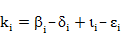. Elements of the community matrix are calculated as:

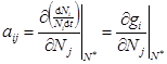
and essentially define the relationships or direct effects between system variables. Alternately, consider the system’s Jacobian matrix (A′), which is derived from the form of Equation (2) (i.e. ). The sign structure of the community and Jacobian matrices are identical, and thus for the purpose of qualitative modelling, either one can be used. Formal quantitative stability analyses, however, require use of the Jacobian matrix, although calculations of perturbation response can proceed with either the community or Jacobian matrix.

As previously discussed, the relationships between variables can be portrayed by signed digraphs, and for our example system with omnivory (Figure 5), the corresponding community matrix:

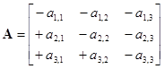
is equivalent in information content to the signed digraph.

A qualitative analysis of local or Lyapunov stability is based on the sign of the eigenvalues () of A, which are the roots of the characteristic equation formed by the equality:

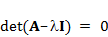
where I is the identity matrix and ‘det’ is the matrix determinant. The resulting characteristic polynomial is of the form:

where 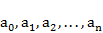, are the system’s polynomial coefficients. A system can be stable if and only if all eigenvalues of A have negative real parts:

For systems with five or more variables, an explicit solution of the roots is not possible, however, conditions for Equation (8) can be ensured through a series of n Hurwitz determinants constructed from the system’s polynomial coefficients:

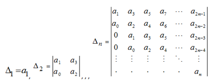
Additionally, a necessary, but not sufficient condition for Equation (8) is that the polynomial coefficients have the same sign. The value of is arbitrarily +1 or –1, and for the convention of equating negative feedback with self damping it can be set equal to –1. This permits an alternative restatement of the conditions for stability via the criteria that: (i) polynomial coefficients are all negative, where ; and, (ii) Hurwitz determinants 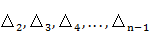all are positive, where .

By these two criteria it is possible to understand stability in terms of the sign and balance of a system feedback (Puccia and Levins, 1985; Dambacher et al., 2003b). The polynomial coefficients describe the feedbacks F at each of n levels in a dynamical system, such that , , 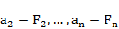. The first criterion requires that feedback at each level be negative such that the system’s dynamics are self damped. Feedback cycles at the first level of a system are composed of the variable’s self-effects. For the example system, there are three feedback cycles at the first level: 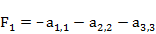. In higher levels of the system, feedback cycles are products of either conjunct or disjunct links. At the second level there are six feedback cycles of length two that are products of either pairwise predator–prey links or the disjunct self-effects. All of these cycles have a negative sign: . Feedback at the highest level of the system is: . Here, there is one positive feedback cycle that involves the benefit that the top predator receives from omnivory. Stability in this system thus depends on the condition that the strength of this positive feedback cycle be less than the sum of the five negatively signed cycles.

The second stability criterion can be generally understood as a balance between higher and lower levels of feedback. A system that is dominated by higher level feedbacks can exhibit over correction and thus be prone to undamped oscillations. For a three-variable system the second criterion is:

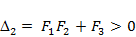
which for our example system requires Here stability depends on the feedback cycle with the negative effect that the basal species receives from omnivory be less than the sum of all other feedback cycles of length three and the products of lower level feedbacks. Stability in this system thus depends on the relative weakness of the omnivory interaction. Moreover, it can be inferred that if omnivory did not occur, then there would be no conditions for instability, in which case the system would be sign stable.

Any long-term impact on an ecosystem can be interpreted and evaluated as a sustained change in one of the system’s growth parameters. This is the case whether the change comes from within the system via a density-dependent parameter, as in Mendelian selection, or externally by way of a density-independent parameter, as in change coming from the environment or change from management, development or experimental purpose. The Assessment team is interested, then, in predicting change in the equilibrium level of each variable, and, through the implicit function theorem, the solution is by differentiation of Equation (2) with respect to :

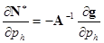
Given the matrix equality:

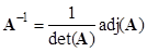
where ‘det’ is the matrix determinant and ‘adj’ is the adjoint matrix, also known as a classical adjoint matrix, Equation (11) can be expressed more conveniently as:

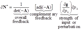
Here is, via Cramer’s Rule (Lay, 2003), the solution for (the difference between the old and new equilibrium abundance for each population), and (the strength or magnitude of a given input or perturbation). For the example system, the solution for the effects of parameter change will be:

From Equation (14) it is evident the matrix A has two separate functions in determining a population’s response to a perturbation. Through the adjoint of A, all direct and indirect effects in the system are combined in complementary feedback cycles (Dambacher et al., 2002), which mediate the relative variation in the response of each population. The determinant of A constitutes the overall feedback of the system and scales the magnitude of each variable’s response to a perturbation. For example, for a given input, if the overall feedback is relatively weak, then the effect of the complementary feedback cycles on population abundance will be relatively large. For this system to be stable requires that det(–A) be positive, and from the above stability analysis, this requires that be relatively weak. Note that use of the determinant of –A maintains a sign convention in the adjoint matrix for even- and odd-sized systems (Dambacher et al., 2002). However, as previously mentioned, system feedback is normally considered to be negative in stable systems; this convention is reversed in Equation (13) and Equation (14) to analyse perturbation response.

In interpreting the adjoint matrix, a positive input to a variable – through an increase in birth rate or decrease in death rate – is read down a column, and response predictions for each variable are read along the rows. Here the correspondence between the matrix adjoint matrix in Equation (14) with the signed digraph analysis in the main text is seen. For a positive input to the prediction of decreased abundance of is determined by two feedback cycles of like sign (i.e. adjoint ), while the ambiguous response of is determined by two feedback cycles of opposing sign (i.e. adjoint). Where inputs to a variable are negative – through a decrease in birth rate or increase in death rate – then the signs of the adjoint matrix elements are simply reversed. In analysis of linear systems, multiple inputs will have an additive effect on the equilibrium of a variable through the superposition principle. Thus if there were simultaneous inputs that increased the birth rate of (e.g. by supplementation) and increased the death rate of (e.g. by culling), then the predicted response of would be calculated as: